Download
1 / 49
490 likes | 609 Views
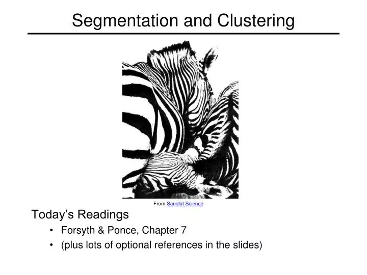
Segmentation and Clustering. Today’s Readings Forsyth & Ponce, Chapter 7 (plus lots of optional references in the slides). From Sandlot Science. From images to objects. What Defines an Object? Subjective problem, but has been well-studied Gestalt Laws seek to formalize this

E N D
Segmentation and Clustering • Today’s Readings • Forsyth & Ponce, Chapter 7 • (plus lots of optional references in the slides) From Sandlot Science
From images to objects • What Defines an Object? • Subjective problem, but has been well-studied • Gestalt Laws seek to formalize this • proximity, similarity, continuation, closure, common fate • see notes by Steve Joordens, U. Toronto
Extracting objects • How could this be done?
Image Segmentation • Many approaches proposed • cues: color, regions, contours • automatic vs. user-guided • no clear winner • we’ll consider several approaches today
Intelligent Scissors [Mortensen 95] • Approach answers a basic question • Q: how to find a path from seed to mouse that follows object boundary as closely as possible?
Intelligent Scissors • Basic Idea • Define edge score for each pixel • edge pixels have low cost • Find lowest cost path from seed to mouse mouse seed • Questions • How to define costs? • How to find the path?
Path Search (basic idea) • Graph Search Algorithm • Computes minimum cost path from seed to allotherpixels
How does this really work? • Treat the image as a graph q c p • Graph • node for every pixel p • link between every adjacent pair of pixels, p,q • cost c for each link • Note: each link has a cost • this is a little different than the figure before where each pixel had a cost
Defining the costs • Treat the image as a graph q c p Want to hug image edges: how to define cost of a link? • the link should follow the intensity edge • want intensity to change rapidly ┴ to the link • c - |difference of intensity ┴ to link|
Defining the costs • c can be computed using a cross-correlation filter • assume it is centered at p • Also typically scale c by its length • set c = (max-|filter response|) • where max = maximum |filter response| over all pixels in the image q c p
1 1 w -1 -1 Defining the costs • c can be computed using a cross-correlation filter • assume it is centered at p • Also typically scale c by its length • set c = (max-|filter response|) • where max = maximum |filter response| over all pixels in the image q c p
9 4 5 1 3 3 3 2 Dijkstra’s shortest path algorithm link cost 0 • Algorithm • init node costs to , set p = seed point, cost(p) = 0 • expand p as follows: • for each of p’s neighbors q that are not expanded • set cost(q) = min( cost(p) + cpq, cost(q) )
9 4 5 1 3 3 3 2 Dijkstra’s shortest path algorithm 4 9 5 1 1 1 0 3 3 2 3 • Algorithm • init node costs to , set p = seed point, cost(p) = 0 • expand p as follows: • for each of p’s neighbors q that are not expanded • set cost(q) = min( cost(p) + cpq, cost(q) ) • if q’s cost changed, make q point back to p • put q on the ACTIVE list (if not already there)
9 4 5 1 3 3 3 2 Dijkstra’s shortest path algorithm 4 9 5 2 3 5 2 1 1 0 3 3 3 4 3 2 3 • Algorithm • init node costs to , set p = seed point, cost(p) = 0 • expand p as follows: • for each of p’s neighbors q that are not expanded • set cost(q) = min( cost(p) + cpq, cost(q) ) • if q’s cost changed, make q point back to p • put q on the ACTIVE list (if not already there) • set r = node with minimum cost on the ACTIVE list • repeat Step 2 for p = r
9 4 5 1 3 3 3 2 Dijkstra’s shortest path algorithm 4 3 6 5 2 3 5 3 2 1 1 0 3 3 3 4 4 3 2 3 • Algorithm • init node costs to , set p = seed point, cost(p) = 0 • expand p as follows: • for each of p’s neighbors q that are not expanded • set cost(q) = min( cost(p) + cpq, cost(q) ) • if q’s cost changed, make q point back to p • put q on the ACTIVE list (if not already there) • set r = node with minimum cost on the ACTIVE list • repeat Step 2 for p = r
Dijkstra’s shortest path algorithm • Properties • It computes the minimum cost path from the seed to every node in the graph. This set of minimum paths is represented as a tree • Running time, with N pixels: • O(N2) time if you use an active list • O(N log N) if you use an active priority queue (heap) • takes fraction of a second for a typical (640x480) image • Once this tree is computed once, we can extract the optimal path from any point to the seed in O(N) time. • it runs in real time as the mouse moves • What happens when the user specifies a new seed?
min cut Segmentation by min (s-t) cut [Boykov 2001] • Graph • node for each pixel, link between pixels • specify a few pixels as foreground and background • create an infinite cost link from each bg pixel to the “t” node • create an infinite cost link from each fg pixel to the “s” node • compute min cut that separates s from t • how to define link cost between neighboring pixels? s t
Is user-input required? • Our visual system is proof that automatic methods are possible • classical image segmentation methods are automatic • Argument for user-directed methods? • only user knows desired scale/object of interest
Automatic graph cut [Shi & Malik] • Fully-connected graph • node for every pixel • link between every pair of pixels, p,q • cost cpq for each link • cpq measures similarity • similarity is inversely proportional to difference in color and position q Cpq c p
w Segmentation by Graph Cuts • Break Graph into Segments • Delete links that cross between segments • Easiest to break links that have low cost (similarity) • similar pixels should be in the same segments • dissimilar pixels should be in different segments A B C
Cuts in a graph • Link Cut • set of links whose removal makes a graph disconnected • cost of a cut: B A • Find minimum cut • gives you a segmentation
Cuts in a graph B A • Normalized Cut • a cut penalizes large segments • fix by normalizing for size of segments • volume(A) = sum of costs of all edges that touch A
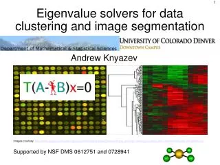
Interpretation as a Dynamical System • Treat the links as springs and shake the system • elasticity proportional to cost • vibration “modes” correspond to segments • can compute these by solving an eigenvector problem • http://www.cis.upenn.edu/~jshi/papers/pami_ncut.pdf
Interpretation as a Dynamical System • Treat the links as springs and shake the system • elasticity proportional to cost • vibration “modes” correspond to segments • can compute these by solving an eigenvector problem • http://www.cis.upenn.edu/~jshi/papers/pami_ncut.pdf
Extension to Soft Segmentation • Each pixel is convex combination of segments.Levin et al. 2006 - compute mattes by solving eigenvector problem
Histogram-based segmentation • Goal • Break the image into K regions (segments) • Solve this by reducing the number of colors to K and mapping each pixel to the closest color
Histogram-based segmentation • Goal • Break the image into K regions (segments) • Solve this by reducing the number of colors to K and mapping each pixel to the closest color Here’s what it looks like if we use two colors
Clustering • How to choose the representative colors? • This is a clustering problem! G G R R • Objective • Each point should be as close as possible to a cluster center • Minimize sum squared distance of each point to closest center
Break it down into subproblems • Suppose I tell you the cluster centers ci • Q: how to determine which points to associate with each ci? • A: for each point p, choose closest ci • Suppose I tell you the points in each cluster • Q: how to determine the cluster centers? • A: choose ci to be the mean of all points in the cluster
K-means clustering • K-means clustering algorithm • Randomly initialize the cluster centers, c1, ..., cK • Given cluster centers, determine points in each cluster • For each point p, find the closest ci. Put p into cluster i • Given points in each cluster, solve for ci • Set ci to be the mean of points in cluster i • If ci have changed, repeat Step 2 • Java demo: http://home.dei.polimi.it/matteucc/Clustering/tutorial_html/AppletKM.html • Properties • Will always converge to some solution • Can be a “local minimum” • does not always find the global minimum of objective function:
K-Means++ • Can we prevent arbitrarily bad local minima? • Randomly choose first center. • Pick new center with prob. proportional to: (contribution of p to total error) • Repeat until k centers. • expected error = O(log k) * optimal • Arthur & Vassilvitskii 2007
Probabilistic clustering • Basic questions • what’s the probability that a point x is in cluster m? • what’s the shape of each cluster? • K-means doesn’t answer these questions • Basic idea • instead of treating the data as a bunch of points, assume that they are all generated by sampling a continuous function • This function is called a generative model • defined by a vector of parameters θ
Mixture of Gaussians • One generative model is a mixture of Gaussians (MOG) • K Gaussian blobs with means μb covariance matrices Vb, dimension d • blob b defined by: • blob b is selected with probability • the likelihood of observing x is a weighted mixture of Gaussians • where
Expectation maximization (EM) • Goal • find blob parameters θthat maximize the likelihood function: • Approach: • E step: given current guess of blobs, compute ownership of each point • M step: given ownership probabilities, update blobs to maximize likelihood function • repeat until convergence
EM details • E-step • compute probability that point x is in blob i, given current guess ofθ • M-step • compute probability that blob b is selected • mean of blob b • covariance of blob b N data points
EM demo • http://lcn.epfl.ch/tutorial/english/gaussian/html/index.html
Applications of EM • Turns out this is useful for all sorts of problems • any clustering problem • any model estimation problem • missing data problems • finding outliers • segmentation problems • segmentation based on color • segmentation based on motion • foreground/background separation • ...
Problems with EM • Local minima k-means is NP-hard even with k=2 • Need to know number of segments solutions: AIC, BIC, Dirichlet process mixture • Need to choose generative model
Finding Modes in a Histogram • How Many Modes Are There? • Easy to see, hard to compute
Mean Shift [Comaniciu & Meer] • Iterative Mode Search • Initialize random seed, and window W • Calculate center of gravity (the “mean”) of W: • Translate the search window to the mean • Repeat Step 2 until convergence
Mean-Shift • Approach • Initialize a window around each point • See where it shifts—this determines which segment it’s in • Multiple points will shift to the same segment
Mean-shift for image segmentation • Useful to take into account spatial information • instead of (R, G, B), run in (R, G, B, x, y) space • D. Comaniciu, P. Meer, Mean shift analysis and applications, 7th International Conference on Computer Vision, Kerkyra, Greece, September 1999, 1197-1203. • http://www.caip.rutgers.edu/riul/research/papers/pdf/spatmsft.pdf More Examples: http://www.caip.rutgers.edu/~comanici/segm_images.html
Choosing Exemplars (Medoids) • like k-means, but means must be data points • Algorithms: • greedy k-means • affinity propagation (Frey & Dueck 2007) • medoid shift (Sheikh et al. 2007) • Scene Summarization
Taxonomy of Segmentation Methods • Graph Based vs. Point-Based (bag of pixels) • User-Directed vs. Automatic • Partitional vs. Hierarchical • K-Means: point-based, automatic, partitional • Graph Cut: graph-based, user-directed, partitional
References • Mortensen and Barrett, “Intelligent Scissors for Image Composition,” Proc. SIGGRAPH 1995. • Boykov and Jolly, “Interactive Graph Cuts for Optimal Boundary & Region Segmentation of Objects in N-D images,” Proc. ICCV, 2001. • Shi and Malik, “Normalized Cuts and Image Segmentation,” Proc. CVPR 1997. • Comaniciu and Meer, “Mean shift analysis and applications,” Proc. ICCV 1999.