Understanding Probability Errors in Sampling: Expected Value and Standard Error
This document explores the concepts of probability errors in sampling, focusing on sample selection, expected value, and standard error. It details examples, such as a survey on marriage among 4,738 freshmen and the implications of sample size on probability errors. It emphasizes using random samples without replacement to reduce bias and discusses how sample size affects error margins, including the use of the normal curve for estimating probabilities. Through empirical data, the text highlights living examples illustrating how sample ratios align with population ratios.

Understanding Probability Errors in Sampling: Expected Value and Standard Error
E N D
Presentation Transcript
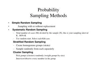
Ch. 15 Probability Errors in Sampling Sample Selection and Probability Error The Expected Value and Standard Error Using the Normal Curve The Correction Factor
1 2 3 4 INDEX Sample Selection and Probability Error The Expected Value and Standard Error Using the Normal Curve The Correction Factor
1. Sample Selection and Probability Error Example • Survey about sense of marriagefrom 4,738 freshmen selecting 100 students (100 samples) After coding each student into different number from 1 to 4,738, select 100 numbers at random by using random number generator. • at random without replacement ☞ no bias
1. Sample Selection and Probability Error Representation of sample Does the Selected samples represents well? (gender ratio of the population: male student 64%) • 250 random samples were drawn from the respondents. The sample size was 100. The number of man in each sample is shown below. Among them the number of getting exactly 64 male students is only 18.
1. Sample Selection and Probability Error Representation of sample • the sample size is 100, histogram of the number of male student (using 250 samples) 15 For the samples selected at random, the percentage of male student goes up or down by chance. 10 % 5 0 49 52 55 58 61 64 67 70 73 76 The number of men As we select samples the probability 64% of drawing male students is not changed, but the probability of being realized in the sample can be changed by the probability error.
1. Sample Selection and Probability Error Sample size and probability error • If we increase the sample size? <sample size is 400> Empirical histogram (R=250) <sample size is 100> Empirical histogram (R=250) The lager the sample size, the less the probability error. (law of averages) (% in the sample) = (% in the population) + (probability error) As the sample size goes up, the sample ratio goes similar to the population ratio.
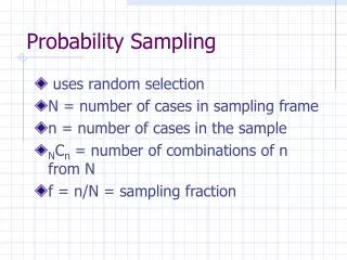
1. Sample Selection and Probability Error Sample Selecting • How can we get as many as 250 samples of which the size is 400 from 4,738? Large circle represents 4,738 people and each shadowed figure represents a sample containing 400 people. Though there are some overlaps, any two of them are not the same. Drawing 400-size samples from 4,738 people There are 4738C400 ways.
1 2 3 4 INDEX Sample Selection and Probability Error The Expected Value and Standard Error Using the Normal Curve The Correction Factor
2. The Expected Value & SE Expected value & SE • With a simple random sample, the expected value for the sample percentage equals the population percentage. • However, the sample percentage will not be exactly equal to its expected value-it will be off by a probability error. ☞ How big is this error likely to be? SE in probability sample represents the standardized size of the probability error.
2. The Expected Value & SE Calculating SE ① Find the SE for the number of men in the sample Making a Box model: There should be only 1’s (male) and 0’s (female) in the box. The number of men in the sample is like the some of 100 draws from the box. (a simple random sample drawn without replacement) SD of box = SE for the sum of 100 draws = (law of square roots) ② Convert to percent, relative to the size of the sample SE for percentage (%) = (SE for number)/(sample size) 100% = 4.8/100 100%=4.8% The SE for the percentage of men in a sample of 100 would be 4.8%
2. The Expected Value & SE Expexted value & SE • What happens as the sample gets bigger? ☞ Law of square roots! • The SE for the sample number goes up like the square root of the sample size. • The SE for the percentage goes down like the square root of the sample size.
1 2 3 4 INDEX Sample Selection and Probability Error The Expected Value and Standard Error Using the Normal Curve The Correction Factor
3. Using the Normal Curve Example 1 A company has 1,000,000 clients. Taking a simple random sample of 400 of them as a part of market research study. 20% of the clients earn over \40,000,000 per year. ① expected value of the percentage Over than \40 million =1, others=0 Expected value of box =0.2 , sum=4000.2=80, Expected value of percentage = (80/400)100=20% The percentage of high earners in the sample will be around 20%, give or take 2% or so. ② the SE of the percentage SD of box = SE for the sum = SE for the percentage =(8/400)100=2% When drawing at random from a box of 0’s and 1’s, the expected value for the percentage of 1’s among the draws equals the percentage of 1’s in the box.
3. Using the Normal Curve Example 2 Estimate the probability that between 18% and 22% of the persons in the sample earn more than \40 million a year The expected value for the percentage is 20% and the SE is 2% now convert 2 standard units. Then probability of shaded area is about 68%.
1 2 3 4 INDEX Sample Selection and Probability Error The Expected Value and Standard Error Using the Normal Curve The Correction Factor
4. The Correction Factor Accuracy of the estimation of percentage Estimating the percentage of voters who are Democratic 1.2 million eligible voters in New Mexico, and about 12.5 million in the state of Texas. Simple random sampling of 2500 voters from each state without replacement. • For which poll is the probability error likely to be smaller? The New Mexico Poll is sampling one voter out of 500 while Texas poll is only sampling one voter out of 5,000. However, it does seem that New Mexico poll should be more accurate then the Texas poll. But, in fact, the accuracies are about the same. Because the two samples of 2500 provide with similar amount of information. When estimating percentages, it is the absolute size of the sample which determines accuracy, not the size relative to the population. This is true if the sample is only a small part of the population, which is the usual case.
drawing with replacement drawing without replacement There is no difference between Drawing from the two boxes. At each trial, the probability of Drawing 0 or 1 is 50 to 50, and the box size does not matter. The number of tickets drawn is Much smaller than the number In the box. So the ratio is almost The same even if we do not replace 4. The Correction Factor The size of population and accuracy Democrats(1=50%) others (0=50%); Two boxes: NM, TX Drawing 2,500 at random from each box with the with replacement: Because the ratio of 1’s equal to 50% and the sizes of sample are same, the SE of the Democrats equal. • If the population size is large enough, it has nothing to do with the accuracy of the estimate
4. The Correction Factor drawing with replacement & drawing without replacement When drawing without replacement, the box gets a bit smaller, reducing the variability slightly. So, the SE for drawing without replacement is a little less then the SE for drawing with replacement. (SE when drawing without replacement)= (SE when drawing with replacement) (correction factor) Correction factor = Number of cards in the box Correction factor 5,000 0.70718 10,000 0.86607 100,000 0.98743 500,000 0.99750 1,000,000 0.99875 12,500,000 0.99990 *n = # of drawn cards = 2,500 (fixed)
4. The Correction Factor The correction factor • When the number of tickets in the box is large relative to the number of draws, the correction factor is nearly 1 can be ignored. • It is the absolute size of the sample which determines accuracy, through the SE for drawing with replacement. The size of the population of the population does not really matter.