Model Order Reduction
Model Order Reduction. Bo Hu Mixed Signal CAD Electrical Engineering Department University of Washington. Outline. Overview of the problem Linear Model Order Reduction Non-linear Model Order reduction Reference. The Problem. Slow to simulate. x(t). u(t). y(t). N is Large. reduce.

Model Order Reduction
E N D
Presentation Transcript
Model Order Reduction Bo Hu Mixed Signal CAD Electrical Engineering Department University of Washington
Outline • Overview of the problem • Linear Model Order Reduction • Non-linear Model Order reduction • Reference
The Problem Slow to simulate x(t) u(t) y(t) N is Large reduce u(t) y(t) z(t) q<<N Fast to simulate
Model Order Reduction • Model Order Reduction: Construct a simplified system to approximate the original system with reasonable accuracy.
Linear Model Order Reduction Reduction Methods are mature for Linear System • Typical application: RC, RL,LC, and RLC circuits. • Speed-up: 10 to 100 or more, depends on problems
Linear Model Order Reduction con't • Basic Idea: Construct a reduced order system whose transfer function Hr(s) is a pade approximation to the transfer function H(s) of the original system. • Why Pade ?
Approximation methods • Taylor Series • Pade Approximations • Lagrange Polynomials • Spline • ... Many other approximations • The choice depends on specific problem
Pade Method con't • The Dynamic System’s transfer function has the following structure: H(s) = A(s)/B(s), for such kind of function, Pade approximation is simple and often better !
Pade Based Algorithm • Moment Matching: • Construct Pade Function Hq(s) to approximate H(s), such that their first q moments are the same
Moment matching methods • Asymptotic Waveform Evaluation(AWE) (Explicit moment matching) • Arnoldi Algorithm(Implicit) • Lanczos algorithm(Implicit)
AWE Method--Explicit moment-matching algorithm • Developed by Pillage, Rohrer in 1990. • Basic Idea: compute the first 2q moments of the transfer function H(s), and then find the pade approximation function Hr(s) to match those 2q moments . • using Hr(s), we can do frequency domain analysis and time domain analysis of the system. • Advantages: easy to understand and implement, when q is small, AWE gives good results.
AWE Process for SISO • Compute the first 2q moment of H(s)
AWE Process for SISO con’t Solve the coefficients of Hq(s) based on the 2q-1 moments of H(s)
AWE for MIMO AWE for MIMO system(m-input,p-output): • get pade approximation separately for each pair of inputs and outputs; • then apply the superposition property of linear networks, group them into one matrix Hq(s); • However the computation cost increase quadraticly with the number of ports:O(m x p).
Numerical problem in AWE Process • AWE gives good result when q<=10 • Beyond that, AWE has numerical instability problem. • The reason is that: when compute the coefficients ai and bi of Hr(s), the AWE method encounter ill-conditioned matrix M.
Arnoldi Algorithm • Developed by Silveira, Kamon, White, Elfadel, Ling etc. in 1990. • Basic Idea: Perform variable substitution x=Vz, such that the reduced system has a transfer function Hq(s) Pade-Approximate to original transfer function H(s). • The construction of V in Arnoldi algorithm is a modified Gram-Schmidt Process
Notes about Arnoldi method • Arnoldi algorithm is a modified Gram-Schmidt process on Krylov subspace • Hq(s) from Arnoldi method matches up to the qth moments. • In Arnoldi algorithm, A= -inv(G)C; When compute V = AR, the practical implementation is:
PRIMA • Passive Reduced Order Interconnect Macromodeling Algorithm: combination of moment matching with congruence transformation. • The advantage of PRIMA: be able to preserve the passivity during the reduction process and in the same time, numerically stable. • Compared to Lanczos algorithm, PRIMA trades part of the accuracy for Passivity, Lanczos algorithm is more efficient, but could lose Passivity.
PRIMA and Passivity • A circuit is passive if none of its elements generates energy. • A system is passive iff
PRIMA • Use Arnoldi Process to obtain V, and perform variable substitution: x = Vz • In the same time, perform congruence transformations as follows:
PRIMA • PRIMA is useful, especially when the system has both linear and nonlinear part • The linear part can be reduced and keep passivity, which is very important for the stability of the dynamic system. Nonlinear Nonlinear reduce Linear Linear
Pade Via Lanczos(PVL) --Another implicit moment matching algorithm • Basic Idea: Implicitly Match first q moment of H(s) by Lanczos Process. • Developed by Feldmann and Freund in1995 • Advantage: Numerically more stable and computationally efficient. • Disadvantage: for RLC system, it does not keep passivity.
Lanczos algorithm overview • Originally Developed by Lanczos at 1950s to solve eigenvalue problems. • Basic Idea: Given matrix A(N by N), and starting with given nonzero vectors r,l (N by 1), run the lanczos process for n steps to obtain matrix Tn(n x n, typically n<<N), Tn is often a very good approximation to matrix A, and Tn’s eigenvalue is close to A’s eigenvalue.
Lanczos Algorithm Application Applications of Lanczos algorithm: • Compute the approximate eigenvalue of matrix A • Solve large systems of linear equations: Ax = b • Used in PVL Algorithm since 1990's.
Lanczos Algorithm for SISO • For SISO system: • Run Lanczos Process, we obtain Tq, and the qth Pade-Approximation to Hq(s) is obtained as follows(e1 is the first unit vector of N by 1):
MPVL Algorithm Outline--with deflation and look-ahead technique • MPVL: multi input and multi output PVL. • Basic idea: after variable transformation x=Vz, the reduced system’s transfer matirx Hr(s) is pade-approximation to original system’s transfer matrix H(s).
MPVL Algorithm Outline con’t--with deflation and look-ahead technique • Practical implementation of MPVL is similar to SISO PVL, • But MPVL requires deflation and look-ahead techniques
MPVL Algorithm Outline--with deflation and look-ahead technique • Deflation procedure: detect and delete linearly dependent or almost linearly dependent vectors in the block Krylov subspace. • For example: if the kth vector in Krylov{A,r} can be represented by the former k-1 vectors, then the kth vector should be deleted from Krylov{A,r}—this procedure is called deflation. • After deflation, the size of Krylov{A,r} and Krylov{A’,l’}may be different, the MPVL process terminates when either Krylov subspace is exhausted.
MPVL Algorithm Outline con’t--with deflation and look-ahead technique • Break-down in lanczos process could happen when vi and wi are orthogonal or almost orthogonal to each other. • Look-ahead technique must be taken to remedy break-down in lanczos process.
MPVL Algorithm Outline con’t--with deflation and look-ahead technique
Comparison of Three methods • AWE is more straight forward to understand and implement, but it is numerically unstable. • Lanczos algorithm is numerically stable, and efficient; but can lose passivity. • Improved Arnoldi method(PRIMA) is stable, and keep the passivity.
Computational cost • The computation cost for the three methods are all under O(N^3), depends on how sparse those coefficient matrices are • Better than solve it directly which requires O(N^4) in general
Nonlinear model order reduction • The problem(m inputs and p outputs)
Available Approaches • Linearization method • Quadratic method • Piece-wise-linear method • Balancing technique
Linearization method • Expand f(x) to first order, and convert the non-linear problem as linear problem • Disadvantage: it strongly depends on how f(x) is similar to a linear function.
Quadratic method • Basic idea: expand f(x) to second order: • Disadvantages: depends on how closely f(x) is similar to quadratic function.
Piece-Wise-Linear method • Basic idea: represent the non-linear system with a piecewise-linear system and then reduce each of the pieces with linear model reduction methods. • Procedure: supply a “training input”, trace the trajectory of the non-linear system, and in the same time generate a set of piecewise linear systems as an approximation to the original non-linear system. x(t) the exact trajectory ---- the pwl approximation t The response to a “training input”
Piece-Wise-Linear method con’t • Works better than linear-reduction and quadratic reduction method. • Disadvantages: the resultant piece-wise-linear system’s accuracy depends on the training input; not qualified as a general approach.
Reference [1] A Trajectory Piecewise linear Approach to model order reduction and fast simulation of nonlinear circuits and micromachined devices, Rewienski; White,J [2] A quadratic method for nonlinear model order reduction, chen,Y; white,J [3] Model Order Reduction for Nonlinear System, Y.Chen [4] PRIMA: Passive reduced order interconnect macromodeling algorithm, Odabasioglu [5] Reduced-order modeling of large linear passive multi-terminal circuits using matrix-Pade approximation, Freund [6] Asymptotic waveform evaluation for timing analysis ,Pillage, L.T.; Rohrer, R.A [7] Feldmann, P. and Freund, R. W., Efficient Linear Circuit Analysis by Pade Approximation via the Lanczos Process [8] Pade approximants / George A. Baker, Jr., Peter Graves-Morris [9] Reduced-order modeling of large linear subcircuits via a block lanczos algorithm, Feldman, Freund [10] A lanczos-type method for multiple starting vectors, Freund,hernandez,boley,aliaga [11] Reduced-Order Modeling Techniques Based on Krylov Subspaces and Their Use in Circuit Simulation, Freund [12] A Block Rational Arnoldi Algorithm for Multipoint Passive Model-Order Reduction of Multiport RLC Networks, Elfadel, Ling

