Download
1 / 38
380 likes | 535 Views
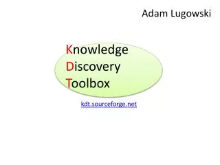
Adam Lugowski. kdt.sourceforge.net. K nowledge D iscovery T oolbox. Our users: Domain Experts. 2. 1. 4. Build input graph. 3. Cull relevant data. Interpret results. Analyze graph. KDT. Data filtering technologies. Graph viz engine. Example workflow. How to target Domain Experts?.

E N D
Adam Lugowski kdt.sourceforge.net • Knowledge • Discovery • Toolbox
Our users: Domain Experts 2 1 4 Build input graph 3 Cull relevant data Interpretresults Analyze graph KDT Datafilteringtechnologies Graphvizengine
How to target Domain Experts? • Conceptually simple • Customizable • High Performance
Complex methods centrality(‘approxBC’) pageRank cluster(‘Markov’) contract . . . Building blocks Mat DiGraph • Vec • SpMV • SpGEMM • load, eye • reduce, scale • +, [] • max, norm,sort • abs, any, ceil • range, ones • +,-,*,/,>,==,&,[] • bfsTree,neighbor • degree,subgraph • load,UFget • +, -, sum, scale Underlying infrastructure (Combinatorial BLAS) • SpMV, SpMV_SemiRing • SpGEMM, SpGEMM_SemiRing Sparse-matrix classes/methods (e.g., Apply, EWiseApply, Reduce) • Algorithm Experts • Domain Experts • HPC Experts
# the variable bigG contains the input graph # find and select the giant component comp = bigG.connComp() giantComp= comp.hist().argmax() G = bigG.subgraph(comp==giantComp) 1. Largest Component
2. Markov Clustering # cluster the graph clus = G.cluster(’Markov’)
3. Graph of Clusters # contract the clusters smallG = G.contract(clus)
Example workflow KDT code # the variable bigG contains the input graph # find and select the giant component comp = bigG.connComp() giantComp= comp.hist().argmax() G = bigG.subgraph(comp==giantComp) # cluster the graph clus= G.cluster(’Markov’) # contract the clusters smallG= G.contract(clus)
BFS on a Scale 29 RMAT graph (500M vertices, 8B edges) Machine: NERSC’s Hopper
2 1 4 5 7 6 3 Breadth-First Search G
2 1 4 5 7 6 3 Breadth-First Search G fin distance 1 from vertex 7
2 1 4 5 7 6 3 Breadth-First Search G fin fout × = distance 1 from vertex 7
2 1 4 5 7 6 3 Breadth-First Search G fin distance 2 from vertex 7
2 1 4 5 7 6 3 Breadth-First Search G fin fout × = distance 2 from vertex 7
KDT BFS routine # initialization parents =Vec(self.nvert(), -1, sparse=False) frontier =Vec(self.nvert(), sparse=True) parents[root] = root frontier[root] = root # 1st frontier is just the root # the semiringmult and add ops simply return the 2ndarg semiring = sr((lambdax,y: y), (lambdax,y: y)) # loop over frontiers whilefrontier.nnn() >0: frontier.spRange() # frontier[i] = i self.e.SpMV(frontier, semiring=semiring, inPlace=True) # remove already discovered vertices from the frontier. frontier.eWiseApply(parents, op=(lambdaf,p: f), doOp=(lambdaf,p: p==-1), inPlace=True) # update the parents parents[frontier] = frontier
BFS comparison with PBGL Performance comparison of KDT and PBGL breadth-first search. The reported numbers are in MegaTEPS, or 106 traversed edges per second. The graphs are Graph500 RMAT graphs with 2scale vertices and 16*2scale edges.
Plain graph Connectivity only.
(T, F,0) Edge Attributes (semantic graph) (T, F,3) (F, T,1) (T, F,2) (T, T,3) (T, F,0) (T, T,1) (T, F,2) (F, F,0) (F, T,1) class edge_attr: isText isPhoneCall weight (F, T,4) (T, T,5)
Edge Attribute Filter G.addEFilter( lambda e: e.weight > 0) (T, F,3) (F, T,1) (T, F,2) (T, T,3) (T, T,1) (T, F,2) (F, T,1) class edge_attr: isText isPhoneCall weight (F, T,4) (T, T,5)
Edge Attribute Filter Stack G.addEFilter( lambda e: e.weight > 0) G.addEFilter( lambda e: e.isPhoneCall) (F, T,1) (T, T,3) (T, T,1) (F, T,1) class edge_attr: isText isPhoneCall weight (F, T,4) (T, T,5)
Filter implementation details • Filter defined as a unary predicate • operates on edge or vertex value • written in Python • predicates checked in order they were added • Each KDT object maintains a stack of filter predicates • all operations respect filter • enables filter-ignorant algorithm design • enables algorithm designers to use filters
Two filter modes • On-The-Fly filters • predicate checked each time an operation touches vertex or edge • Materialized filters • make copy of graph which excludes filtered elements • predicate checked only once for each element
Performance of On-The-Fly filtervs. Materialized filter • For restrictive filter • OTF can be cheaper since fewer edges are touched • corpus can be huge, but only traverse small pieces • For non-restrictive filter • OTF Saves space (no need to keep two large copies) • OTF Makes each operation more computationally expensive
texts and phone calls # draw graph draw(G) # Each edge has this attribute: class edge_attr: isText isPhoneCall weight
Betweenness Centrality bc = G.centrality(“approxBC”) # draw graph with node sizes # proportional to BC score draw(G, bc)
Betweenness Centrality on texts # BC only on text edges G.addEFilter( lambdae: e.isText) bc = G.centrality(“approxBC”) # draw graph with node sizes # proportional to BC score draw(G, bc)
Betweenness Centrality on calls # BC only on phone call edges G.addEFilter( lambdae: e.isPhoneCall) bc = G.centrality(“approxBC”) # draw graph with node sizes # proportional to BC score draw(G, bc)
SEJITS The way to make Python fast is to not use Python. -- Me • Selective Embedded Just-In-Time Specialization • Take Python code • Translate it to equivalent C++ code • Compile with GCC • Call compiled version instead of Python version
BFS with SEJITS Time (in seconds) for a single BFS iteration on Scale 25 RMAT (33M vertices, 500M edges) with 10% of elements passing filter. Machine is NERSC’s Hopper.
BFS with SEJITS Time (in seconds) for a single BFS iteration on Scale 23 RMAT (8M vertices, 130M edges) with 10% of elements passing filter. Machine is Mirasol.
Roofline • A way to find what your bottleneck is • MEASURE and PLOT potential limiting factors in your exact system and program • compute power • RAM stream speed • RAM random access speed • disk • etc • Your Roofline is the minimum of your plots
KDT + SEJITS Roofline Good (limited by DRAM) Bad (Compute limited)
Is MapReduce any good for graphs? The prospect of the entire graph traversing the cloud fabric for each MapReduce job is disturbing. - Jonathan Cohen
MapReduce-based PageRank comparison with Pegasus Performance comparison of KDT and Pegasus PageRank (ε = 10−7). The graphs are Graph500 RMAT graphs. The machine is Neumann, a 32-core shared memory machine with HDFS mounted in a ramdisk.
A Scalability limit for matrix-matrix multiplication: sqrt(p) Million Traversed Edges Per Second in Betweenness Centrality computation. BC algorithm is composed of multiple BFS searches batched together into matrices and using SpGEMM for traversals.