Download
1 / 44
450 likes | 659 Views
Laboratory Observations of Fast Collisionless Magnetic Reconnection. J. Egedal, J. Dorris, W. Fox, E. Ptacek, M. Porkolab and A. Fasoli MIT Plasma Science and Fusion Center Physics Department. Outline. Magnetic reconnection Generalities, examples and open questions

E N D
Laboratory Observations of Fast Collisionless Magnetic Reconnection J. Egedal, J. Dorris, W. Fox, E. Ptacek, M. Porkolab and A. Fasoli MIT Plasma Science and Fusion Center Physics Department
Outline • Magnetic reconnection • Generalities, examples and open questions • Driven reconnection in the VTF open cusp • Dynamic evolution of j and E. • j||and dE/dt linked through ion-polarization • Size of diffusion region (where EB0) • Orbit effects • Closed cusp configuration, the effect of passing particles. • Conclusions and future work
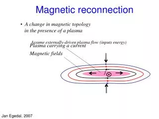
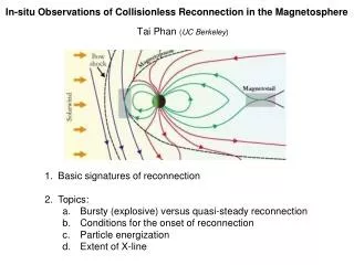
Earth: substorms, aurora Fusion: internal relaxations (strong guide field) Magnetic Reconnection Change in B-field topology in the presence of plasma Sun: flares, coronal mass ejections
B B • h 0: E + v B = hjB can diffuse wrt plasma • tR = m0L2/h resistive time Plasma as a charged fluid • Resistivity h = 0: plasma and B frozen together
Need to model local geometry (1957) Sweet-Parker model (1964) Petschek model (1971) Turbulence, B. Coppi & A. Friedland Reconnection is an open question(1) resistive time tRobserved time for reconnection tokamaks 1-10 s10-100 ms solar flares ~104 years~20 min substorms ~infinite~30 min
2D w/ walls 2D Symmetry global boundary local steady state process transient collisionality collisionless collisional Family of Reconnection Experiments (H.Ji, PPPL)
Magnetic Reconnection on VTF The VTF device 2 m • Change in B-field topology in a plasma • Need to understand • Origin of fast time scale for reconnection • Particle orbits ? • Instabilities / waves ?
Primary Diagnostics 45 heads L-probe 40 Channels B-probe
Ex. of target plasma profiles Bcusp = 50mT, Bguide= 87mT; PECRH ~ 30 kW VTF configuration • lmfp>>L, tcoll>torbit,tA;ri<<L • S = m0LvA/h>>1 • Plasma production by ECRH separate from reconnection drive J.Egedal et al., RSI 71, 3351 (2000)
Reconnection drive • Ohmic coils driven by LC resonant circuit • Flux swing ~ 0.2 V-s, duration ~ 6 ms (>>trec) • Vloop ~ 100 V, vExB ~ 2km/s ~ vA/10
Sketch of poloidal flux during reconnection drive No reconnection as in ideal MHD Fast reconnection as in vacuum
Ideal region: E + v×B= 0 E · B = 0 - Ez -l0 l0 2x 2y Electrostatic potential (away from the X-line) E= Ezz - B=b0 ( x x – y y + l0 z) =½Ezl0log(|x/y|) E = Ez ( x + y + z) ? ?
Experimental potential The size of the diffusion region Frozen in law is broken where EB0 EB=(E -) B a = 3.5 cm
Neon Nitrogen Krypton Xenon • The size depends • on [cm] The size of the diffusion region • The size of the • diffusion region is • independent of ion • mass and number • density.
Temporal evolution of the current channel Time response of the toroidal current Eigen response, f= 10-30 kHz
In phase withVloop 900 ahead of Vloop 0 – 1.2 kA/(Vm2) 0 – 20 mAs/(Vm2) Plasma response to an oscillating drive • The current profile • can be separated in • two parts:
Ion polarization currents due to d/dt Ion polarization current: Quasi neutrality: , = 3.5 cm
, , Circuit model for VTF plasmas
The scaling is • verified when using • Empirical scaling: Cj2Vloop Cj2Vloop [As] [As] Circuit model for VTF plasmas • Total current is measured in each • shot by a Rogowsky coil • Values of R j1 and Cj2 obtained • by curve fitting
What breaks the frozen in condition? The plasma frozen in condition is violated where: Generalized Ohms law:
[cm] Breaking the frozen in law • All electrons are trapped • limiting macroscopic current channel • Electrons short circuit electric • fields along their orbits • The frozen in law is broken in areas • where the orbits do not follow the • field lines: E•B0 Orbit width, cusp= (g l0)0.5 J.Egedal, PoP 9, 1095 (2002)
Density Assume a Maxwell dist. for (x,y)=6 l0 : p||/p Drift kinetic calculation Linear cusp, B=b0(xx-yy+l0z), Az=b0xy-Ezt, =½Ezl0log(x/y) • Conserved quantities: • = mv2/(2B) J = v dl (=v||/v) J.Egedal, PoP 9, 1095 (2002)
Electron Hybrid Probe: • Invented by Khash Shadman. • A probe compatible with VTF plasmas • was implemented by James Dorris. • The probe provides information about • the rotational energy of the electron as • a function of v||. I [A] t [s]
Drift kinetic modeling • Recent Wind satellite observation: • Strong anisotropy in f near X-line • This anisotropy was predicted by the • drift kinetic modeling • The magnetic moment is not • conserved for energies above 1keV • Good agreement with observation when • including pitch angle diffusion M. Øieroset et al. PRL 89, (2002)
Boundary conditions New configuration: Closed cusp passing particles
Boundary conditions Open cusp: Closed cusp:
Future research in VTF • The closed configuration provides boundary conditions and • plasma parameters ideal for our future research on reconnection VTF closed cusp
Conclusions • Fast, collisionless driven reconnection observed in the open cusp configuration • Dynamic evolution of the current profile and the self-consistent plasma potential observed for the first time during reconnection • LCR circuit accounts for the time behavior of the toroidal plasma current • Classical collisions are not important • The width of the diffusion region scales with cusp • Toroidal current limited due to trapped orbits pe, dJ/dt • New closed cusp configuration, suitable for future research • Strong current throughout the cross section. • The closed geometry will be used in our future research on collisionless reconnection
What breaks the frozen in condition? Anomalous resistivity, , is incompatible with observations j|| E||
Drift kinetic calculation (2) Characteristics in (x,)-space ~ ~ ~ • = v 2 g1; g1 (x,)=(1-2)/(2B) • J = v g2; g2 (x,) = dl • /J2 = g1 (x,)/[g2 (x,)] 2 • is a COM contours are • characteristics through the • (x,)-plane • Consider two points on a characteristic: • (v1,x1,1) and (v2,x2,2 ): • v12g1 (x1,1) = v22g1(x2,2) • v1/v2 = [g1(x2,2) / g1(x1,1)]½ • = h(x1,1,x2) h(x1,1), for x2=6l0
Future developments • Full high resolution reconstruction of j(x,t), Y(x,t), E(x,t), n(x,t) and v(x,t) in different Bcusp/Bf regimes (probe upgrades) • Scaling of the size of the diffusion region with Bcusp,, Bf • Direct measurements of off diagonal elements in pe • Direct measurements of ion heating • Machine upgrades • Increase strength of reconnection drive • Reinstallation of in-vessel coils
Drift kinetic calculation (4) • Flows: • v= E B / B2 • obtain v|| • from div(nv)=0
Linear cusp, B=b0 ( x x – y y + l0 z) E= Ezz - , Drift kinetic modeling • For a given electric and magnetic geometry, the • collisionless drift kinetic equation dfg/dt=0 may be solved by • the methods of characteristics. • The characteristics are the guiding center orbits. • The electric and magnetic geometry is obtained from the • experiment: • Particles are propagated back in time to a • point where fg is assumed to be Maxwell • distributed.
Itot E J(r) n(r) Current sheet, electric field, density, and potential evolution for weak Ip Vfloat(r) plasma slows down reconnection
Two fluid model for VTF (J.Ramos, F.Porcelli) • Strong Bguide, low b, boundaries at , T=const, p isotropic • Grad(p) (rS) and /tJ (de) terms are important • Current decay: transition from collisionless to collisional • Agrees with • Self-consistent potential away from separatrix • Absence of steady-state current layer. • Disagrees with • Time evolution of E, E hJ even for t • Large diffusion region observed in experiment
VTF Diagnostics: LIFE.g. planar set-up: fi(vklaser,x,y) • Pulsed dye laser (Lambda Physik Scanmate pumped by Nd:Yag) pumps 611.5 nm line Elaser ~ 20 mJ in 10 ns • LIF detected at 461 nm (intensified CCD?) 2 1 3