Download
1 / 31
350 likes | 591 Views
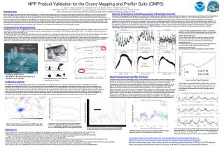
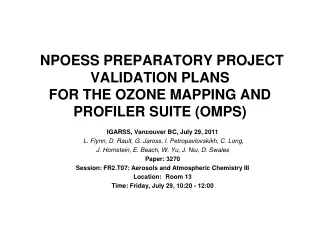
Measuring the Antarctic Ozone Hole with the new Ozone Mapping and Profiler Suite (OMPS). Natalya Kramarova, Paul Newman, Eric Nash, PK Bhartia, Richard McPeters , Didier Rault, Colin Seftor, Gordon Labow. OMPS meeting, June 6, 2013. Can OMPS reasonably represent the Antarctic ozone hole?

E N D
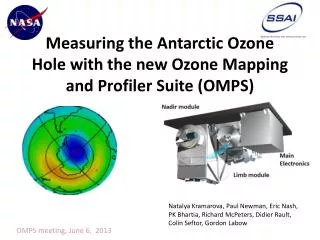
Measuring the Antarctic Ozone Hole with the new Ozone Mapping and Profiler Suite (OMPS) Natalya Kramarova, Paul Newman, Eric Nash, PK Bhartia, Richard McPeters, Didier Rault, Colin Seftor, Gordon Labow OMPS meeting, June 6, 2013
Can OMPS reasonably represent the Antarctic ozone hole? • Do the metrics derived from OMPS match OMI and MLS? • Is OMPS an improvement? Objectives OMPS meeting, June 6, 2013
I. Introduction II. The Ozone Mapping and Profiler Suite (OMPS) III. Validation of OMPS measurements IV. OMPS ozone hole first results V. Conclusions Outline: OMPS meeting, June 6, 2013
III. Validation of OMPS measurements September –November 2012 Biases increase for higher latitudes OMPS NP vs OMPS LP Coincidence criteria: +/-0.5 hour, +/-1° latitude, +/-4° longitude. OMPS meeting, June 6, 2013
III. Validation of OMPS measurements September –November 2012 OMPS NP overestimates ozone compared to SBUV SBUV vs OMPS NP Coincidence criteria: +/-4 hour, +/-1° latitude, +/-5° longitude. OMPS meeting, June 6, 2013
III. Validation of OMPS measurements September –November 2012 OMPS LP vs Aura MLS Coincidence criteria: +/-1 hour, +/-1° latitude, +/-4° longitude. OMPS meeting, June 6, 2013
III. Validation of OMPS measurements September –November 2012, 36 balloon measurements OMPS LP and Aura MLS vsNeumayerSonde (70.6S, 8W) Coincidence criteria: 1000-km distance from the station (dist. weight. average); same day. OMPS meeting, June 6, 2013
III. Validation of OMPS measurements SONDE SONDE Aura MLS/OMPS LP vsNeumayerSonde Aura MLS OMPS LP OMPS meeting, June 6, 2013
III. Validation of OMPS measurements Total ozone column comparisons OMPS TC vs OMPS NP • Biases < 1% • Standard deviation is 3-4% OMPS NP vs SBUV NOAA18 OMPS NP vs SBUV NOAA19 OMPS meeting, June 6, 2013
Total ozone, October 2012 IV. OMPS ozone hole first results OMPS meeting, June 6, 2013
Total ozone, October 2012 Low values generally found inside ozone hole IV. OMPS ozone hole first results Higher values found outside ozone hole everywhere OMPS meeting, June 6, 2013
IV. OMPS ozone hole first results OMPS compares quite well with OMI, but slightly smaller because of the high bias 2012 Antarctic ozone hole was 2nd smallest observed in the last twenty-three years — only the major warming 2002 ozone hole was smaller Area of the Antarctic ozone hole based on TOMS and OMI measurements. Red bar shows an estimate from OMPS TC. OMPS meeting, June 6, 2013
IV. OMPS ozone hole first results Area Evolution of 2012 Antarctic ozone hole More rapid disappearance after mid-September Minimum “Normal” development up to mid-September OMPS meeting, June 6, 2013
IV. OMPS ozone hole first results OMPS meeting, June 6, 2013
IV. OMPS ozone hole first results OMPS meeting, June 6, 2013 Location of the ozone hole center for September, October, and November
IV. OMPS ozone hole first results OMPS meeting, June 6, 2013 Total ozone values following the ozone hole
IV. OMPS ozone hole first results OMPS meeting, June 6, 2013 Ozone profile following the ozone hole’s center
IV. OMPS ozone hole first results OMPS meeting, June 6, 2013 Strong depletion of ozone in the 14-24 km region
IV. OMPS ozone hole first results Lowest total ozone value reached about Oct. 1 OMPS meeting, June 6, 2013
IV. OMPS ozone hole first results OMPS meeting, June 6, 2013 Lowest profile value reached about Oct. 11
IV. OMPS ozone hole first results Strong build-up of ozone in the middle stratosphere leads to overall ozone increase OMPS meeting, June 6, 2013
IV. OMPS ozone hole first results Large ozone loss sharpens the vertical gradient. The gradient’s altitude is related to the Cl levels. As Cl declines, the gradient should move to lower altitudes. OMPS meeting, June 6, 2013
IV. OMPS ozone hole first results OMPS meeting, June 6, 2013
IV. OMPS ozone hole first results Clear signs of ozone depletion in the upper layer + + High ozone concentration in the lowermost stratosphere + = OMPS meeting, June 6, 2013
IV. OMPS ozone hole first results The 3 layers show depletions by mid-September Deep ozone hole OMPS meeting, June 6, 2013
IV. OMPS ozone hole first results Area of the hole decreases Deep ozone hole Total ozone min ~ 1 Oct. OMPS meeting, June 6, 2013
IV. OMPS ozone hole first results Notable decrease of the hole area in middle and upper stratosphere Min ozone at mid Oct Signs of ozone recovery OMPS meeting, June 6, 2013
IV. OMPS ozone hole first results Ozone hole splits OMPS meeting, June 6, 2013
IV. OMPS ozone hole first results • Ozone increasing in all 3 layers • Total ozone shows a rapid increase by late-November OMPS meeting, June 6, 2013
V. Conclusions (1) • OMPS suite began routine operations in 2012. • OMPS is derived from the strong heritage of UV-Vis satellite instruments that extend from the 1970s; • Will become the standard ozone monitoring instrument aboard the US polar orbiting satellites. • OMPS performs quite reasonably. • direct comparisons of OMPS TC to the OMI column observations show differences of <1%; • comparisons of the ozone profiles obtained from OMPS LP and NP with the profiles from the Aura MLS, SBUV, and ozone sondes show good agreement (biases <5-8% and std dev <5-10%) in the vertical range 20-45 km; • good agreements between OMPS TC and OMI on estimates of the average minimum ozone and ozone hole area. OMPS meeting, June 6, 2013
V. Conclusions (2) • 2012 ozone hole • 2nd smallest since 1988 - weakest ozone hole was 2002 – driven by the first observed major SSW observed in the SH; • Early development (Aug. to mid-Sep.) was normal – still plenty of Cl and Br for ozone loss. In the lower stratosphere, large losses seen in the LP from early Sep. to about 11 Oct. Ozone near zero at 16 km altitude by Oct. 11. Lowest columnseen about Oct.1. Very strong vertical gradient develops by early October; • Extremely high values of ozone seen in upper stratosphere by Mid-October as ozone is advected over Antarctica; • Ozone hole disappeared (late-Sep to Nov) quite rapidly in comparison to the ozone holes in the last 20-year period, because of the strong wave dynamics, faster warming during Austral spring, and stronger advection. OMPS meeting, June 6, 2013