Download

1 / 16
170 likes | 295 Views
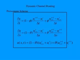
Dynamic Channel Routing. Preissmann Scheme. Dynamic Channel Routing. Preissmann Scheme. unconditionally stable for q >=0.5 second-order accurate if q = f = 0.5, first order otherwise not valid for transcritical flow variations of Preissman scheme used in many models.

E N D
Dynamic Channel Routing Preissmann Scheme
Dynamic Channel Routing Preissmann Scheme • unconditionally stable for q>=0.5 • second-order accurate if q = f = 0.5, first order otherwise • not valid for transcritical flow • variations of Preissman scheme used in many models focus on FLDWAV here...
Assumptions in St. Venant Equations • Flow is 1-D: flow characteristics (depth, velocity, etc.) vary only in the longitudinal x-direction of the channel. • Water surface is horizontal across any section perpendicular to the longitudinal axis. • Flow is gradually varied with hydrostatic pressure prevailing at all points in the flow. • Longitudinal axis of the channel can be approximated by a straight line. • Bottom slope of the channel is small, i.e., tan h = sin h. (h =10% yields 1.5% variation). • Bed of the channel is fixed, i.e., no scouring or deposition is assumed to occur. • Resistance coefficient for steady uniform turbulent flow is considered applicable and an empirical resistance equation such as the Manning equation describes the resistance effect. • Flow is incompressible and homogeneous in density.
Continuity Momentum
Dt Momentum Continuity Dx Computational Grid t 1 2 3 4 5 6 7 DOWNSTREAM BOUNDARY Flow, WSEL, or tide T.S or Rating Curve UPSTREAM BOUNDARY Flow or WSEL T.S. j+1 j x t=0 i i+1 INITIAL CONDITIONS Initial flow & elevation at each cross section location; Lateral Flow, pool elevation, gate control switch at each location
Matrix Format UB … C1 … M1 … C2 … M2 … C3 … M3 … DB … X X X X X X X X X X X X X X X X X X X X X X X X X X X X Dh1 -RUB -RC1 -RM1 -RC2 -RM2 -RC3 -RM3 -RDB DQ1 Dh2 DQ2 = Dh3 DQ3 Dh4 DQ4 solved using Newton-Raphson method
Local Partial Inertia The s parameter “filters” the inertial terms of the momentum equation based on the Froude number so that this equation transitions between the dynamic and diffusion equation in transition region.
Expanded Equations Basic: DWOPER: off-channel storage, expansion/contraction, lateral inflow, wind: DAMBRK: add sinuosity, mud/debris flow, no wind: FLDWAV: all capabilities above:
Information Requirements Stage-Discharge Relationship Channel Properties: • Geometry • Slope • Roughness Hydrograph Properties: • Peak Flow • Time to Peak Flow • Average Flow
BO = 0 Plan View A River Off-channel storage A Tributary B5 BO5 BO4 B4 B3 Active h B2 Dead Storage B1 Datum Cross Section A-A Plan view of river with active and dead storage areas, and cross section view.
Actual Cross Section B5 HS5 B4 HS4 B3 HS3 B2 HS2 HS1 Each cross section is cast as a top width vs. elevation curve. The shape of the actual cross section is not retained. Top Width vs. Elevation Curve Symmetrical Cross Section Elevation (HS) Top Width (B)
L 1 x 1 Left Floodplain L x 2 2 Floodplains and Sinuosity Main Channel Actual Cross Section B5 BL5 BR5 HS5 B4 BL4 BR4 Right Floodplain HS4 BL3 BR3 B3 HS3 B2 HS2 HS1 The actual cross section is divided into three components: main channel, left floodplain and right floodplain. Each component is modeled as a separate channel using sinuosity and conveyance. Sinuosity Coefficient: s1 = L1/x1
Channel Configurations Single Channel Dendritic (tree-type) System River & Tributaries Canal & Distributaries River Delta Network
FLDWAV Capabilities • Routes outflow hydrograph hydraulically through downstream river/valley system using expanded form of 1-D Saint-Venant equations • Considers effects of: downstream dams, bridges, levees, tributaries, off-channel storage areas, river sinuosity, backwater from tides • Flow may be Newtonian (water) or non-Newtonian (mud/debris) • Produces output of: • a. High water profiles along valley • b. Flood arrival times • c. Flow/stage/velocity hydrographs • Exports data needed to generate flood forecast map: • a. Channel location (river mile and latitude/longitude) • b. Channel invert profile • c. Water surface profile for area to be mapped • d. Channel top width corresponding to water surface elevations in profiles
LQ Q t LQ Q B t B RC RC LEGEND B - bridge RC - rating curve - reservoir and dam - lateral inflow LQ - levee overtopping and/or failure B L - lock and dam manually operated L B Tidal Boundary