Conservation Laws and Nonlinear Hyperbolic PDEs
170 likes | 439 Views
Conservation Laws and Nonlinear Hyperbolic PDEs. Rob Chase and Pat Dragon Under Supervision of Robin Young. Motivation: Conservation laws are replete in Nature. Traffic Patterns Cars are neither created nor destroyed Astronomy Star density Supernovae Fluid Dynamics

Conservation Laws and Nonlinear Hyperbolic PDEs
E N D
Presentation Transcript
Conservation Laws and Nonlinear Hyperbolic PDEs Rob Chase and Pat Dragon Under Supervision of Robin Young
Motivation: Conservation laws are replete in Nature. • Traffic Patterns • Cars are neither created nor destroyed • Astronomy • Star density • Supernovae • Fluid Dynamics • Shallow water wave equations • Euler’s gas dynamic equations
Euler’s Shocktube A long thin tube that allows movement of conserved quantities only in one dimension. (think of a highway) Less Dense More Dense
ODEs involve derivatives with respect to only one variable x’ = 4x (linear) y’ = 4y^2 (nonlinear) PDEs involve partial derivatives with respect to space/time ut + ux = 0 (linear) ut + u*ux = 0 (nonlinear) ODEs vs PDEs
Systems of PDEs ut + f1x(u,v,w)+g1y(u,v,w)+h1z(u,v,w)=0 vt + f2x(u,v,w)+g2y(u,v,w)+h2z(u,v,w)=0 wt + f3x(u,v,w)+g3y(u,v,w)+h3z(u,v,w)=0 Define U = Transpose(u,v,w) Ut + Fx(U) + Gy(U) + Hz(U) = 0 U(0,x,y,z) = Initial Conditions
u= Exp[-x^2] Ut+Fx(U)=0 Two representations of initial conditions: Initial conditions as profiles at time t=0 Initial Conditions = U(0,x) Initial conditions as a curve in statespace parameterized by x u axis x axis v= 1/(x^2+1) v axis x axis w= UnitStep[x] w axis x axis
Hyperbolicty A system is called hyperbolic if the flux matrix F has real eigenvalues. A hyperbolic system is called strictly hyperbolic if the real eigenvalues are all distinct. If the eigenvalues are distinct, then the eigenvectors are independent.
Characteristic Curves Analogous to level curves of surfaces in 3D In linear systems, the characteristics are parallel. In some nonlinear systems, the characteristics intersect forming discontinuities and waves. Characteristics are straight lines unless they interact with waves.
Finding the Eigensystems of PDEs The eigensystem of a flux matrix may be calculated using linear algebra. Finding the eigensystem, the system may be “decoupled” into separate equations for each state variable. The resulting system of ODEs is easier to solve.
This Summer… vt+ fx(v) = 0 v,f scalars W=Transpose(u,z) Wt+[A(v)W]x = 0 The eigensystem of A can be used to find the 3x3 eigensystem. Maintaining Strict Hyperbolicity we will find flux functions and initial data that will “blow up” in finite time but remain “smooth”