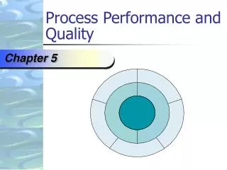
Process Performance and Quality
Chapter 6 explores how process performance and quality contribute to operations management. By leveraging Total Quality Management (TQM) principles, businesses can create a competitive weapon through effective operations strategies. The chapter discusses customer satisfaction, employee involvement, and continuous improvement as key components. It highlights practical applications at Crowne Plaza Christchurch, emphasizing the role of employee empowerment, quality circles, and statistical process control in maintaining high service standards. Understanding and managing costs of poor process performance is crucial for operational excellence.

Process Performance and Quality
E N D
Presentation Transcript
Process Performance and Quality Chapter 6
How Process Performance and Quality fits the Operations Management Philosophy Operations As a Competitive Weapon Operations Strategy Project Management Process Strategy Process Analysis Process Performance and Quality Constraint Management Process Layout Lean Systems Supply Chain Strategy Location Inventory Management Forecasting Sales and Operations Planning Resource Planning Scheduling
Quality at Crowne Plaza Christchurch • The Crowne Plaza is a luxury hotel with 298 guest rooms three restaurants, two lounges and 260 employees to serve 2,250 guests each week. • Customers have many opportunities to evaluate the quality of services they receive. • Prior to the guest’s arrival, the reservation staff gathers a considerable amount of information about each guest’s preferences. • Guest preferences are shared with housekeeping and other staff to customize service for each guest. • Employees are empowered to take preventative, and if necessary, corrective action.
Costs of Poor Process Performance • Defects: Any instance when a process fails to satisfy its customer. • Prevention costs are associated with preventing defects before they happen. • Appraisal costs are incurred when the firm assesses the performance level of its processes. • Internal failurecosts result from defects that are discovered during production of services or products. • External failurecosts arise when a defect is discovered after the customer receives the service or product.
Total Quality Management • Quality: A term used by customers to describe their general satisfaction with a service or product. • Total quality management (TQM) is a philosophy that stresses three principles for achieving high levels of process performance and quality: • Customer satisfaction • Employee involvement • Continuous improvement in performance
Service/product design Process design Continuous improvement Employee involvement Customer satisfaction Problem-solving tools Purchasing Benchmarking TQM Wheel
Customer Satisfaction • Customers, internal or external, are satisfied when their expectations regarding a service or product have been met or exceeded. • Conformance: How a service or product conforms to performance specifications. • Value: How well the service or product serves its intended purpose at a price customers are willing to pay. • Fitness for use: How well a service or product performs its intended purpose. • Support: Support provided by the company after a service or product has been purchased. • Psychological impressions: atmosphere, image, or aesthetics
Employee Involvement • One of the important elements of TQM is employee involvement. • Quality at the source is a philosophy whereby defects are caught and corrected where they were created. • Teams: Small groups of people who have a common purpose, set their own performance goals and approaches, and hold themselves accountable for success. • Employee empowerment is an approach to teamwork that moves responsibility for decisions further down the organizational chart to the level of the employee actually doing the job.
Team Approaches • Quality circles: Another name for problem-solving teams; small groups of supervisors and employees who meet to identify, analyze, and solve process and quality problems. • Special-purpose teams: Groups that address issues of paramount concern to management, labor, or both. • Self-managed team: A small group of employees who work together to produce a major portion, or sometimes all, of a service or product.
Continuous Improvement • Continuous improvement is the philosophy of continually seeking ways to improve processes based on a Japanese concept called kaizen. • Train employees in the methods of statistical process control (SPC) and other tools. • Make SPC methods a normal aspect of operations. • Build work teams and encourage employee involvement. • Utilize problem-solving tools within the work teams. • Develop a sense of operator ownership in the process.
Plan Act Do Check The Deming WheelPlan-Do-Check-Act Cycle
Statistical Process Control • Statistical process control is the application of statistical techniques to determine whether a process is delivering what the customer wants. • Acceptance sampling is the application of statistical techniques to determine whether a quantity of material should be accepted or rejected based on the inspection or test of a sample. • Variables: Service or product characteristics that can be measured, such as weight, length, volume, or time. • Attributes: Service or product characteristics that can be quickly counted for acceptable performance.
Sampling • Sampling plan: A plan that specifies a sample size, the time between successive samples, and decision rules that determine when action should be taken. • Sample size: A quantity of randomly selected observations of process outputs.
Sample Means andthe Process Distribution Sample statistics have their own distribution, which we call a sampling distribution.
where xi = observations of a quality characteristic such as time. n = total number of observations x = mean Sample Mean Sampling Distributions A sample mean is the sum of the observations divided by the total number of observations. The distribution of sample means can be approximated by the normal distribution.
where = standard deviation of a sample n = total number of observations xi = observations of a quality characteristic x = mean Sample Range The range is the difference between the largest observation in a sample and the smallest. The standard deviation is the square root of the variance of a distribution.
Process Distributions • A processdistribution can be characterized by its location, spread, and shape. • Location is measured by the mean of the distribution and spread is measured by the range or standard deviation. • The shape of process distributions can be characterized as either symmetric or skewed. • A symmetricdistribution has the same number of observations above and below the mean. • A skeweddistribution has a greater number of observations either above or below the mean.
Causes of Variation • Two basic categories of variation in output include common causes and assignable causes. • Commoncauses are the purely random, unidentifiable sources of variation that are unavoidable with the current process. • If processvariability results solely from common causes of variation, a typical assumption is that the distribution is symmetric, with most observations near the center. • Assignablecauses of variation are any variation-causing factors that can be identified and eliminated, such as a machine needing repair.
Assignable Causes • The red distribution line below indicates that the process produced a preponderance of the tests in less than average time. Such a distribution is skewed, or no longer symmetric to the average value. • A process is said to be in statistical control when the location, spread, or shape of its distribution does not change over time. • After the process is in statistical control, managers use SPC procedures to detect the onset of assignable causes so that they can be eliminated. Location Spread Shape © 2007 Pearson Education
Control Charts • Control chart: A time-ordered diagram that is used to determine whether observed variations are abnormal. A sample statistic that falls between the UCL and the LCL indicates that the process is exhibiting common causes of variation; a statistic that falls outside the control limits indicates that the process is exhibiting assignable causes of variation.
Type I and II Errors • Control charts are not perfect tools for detecting shifts in the process distribution because they are based on sampling distributions. Two types of error are possible with the use of control charts. • Type I error occurs when the employee concludes that the process is out of control based on a sample result that falls outside the control limits, when in fact it was due to pure randomness. • Type II error occurs when the employee concludes that the process is in control and only randomness is present, when actually the process is out of statistical control.
Statistical ProcessControl Methods • Control Charts for variables are used to monitor the mean and variability of the process distribution. • R-chart (Range Chart) is used to monitor process variability. • x-chart is used to see whether the process is generating output, on average, consistent with a target value set by management for the process or whether its current performance, with respect to the average of the performance measure, is consistent with past performance. • If the standard deviation of the process is known, we can place UCL and LCL at “z” standard deviations from the mean at the desired confidence level.
– The control limits for the R-chart are UCLR = D4R and LCLR = D3Rwhere R = average of several past R values and the central line of the chart.D3,D4 = constants that provide 3 standard deviations (three-sigma) limits for a given sample size. Control Limits The control limits for the x-chart are: UCLx= x + A2R and LCLx = x - A2R Where X = central line of the chart, which can be either the average of past sample means or a target value set for the process. A2 = constant to provide three-sigma limits for the sample mean. = = – =
Calculating Three-Sigma Limits Table 6.1
West Allis Industries Example 6.1 West Allis is concerned about their production of a special metal screw used by their largest customers. The diameter of the screw is critical. Data from five samples is shown in the table below. Sample size is 4. Is the process in statistical control?
Special Metal Screw Sample Sample Number 1 2 3 4 Rx 1 0.5014 0.50220.5009 0.5027 0.0018 0.5018 2 0.5021 0.5041 0.5024 0.5020 3 0.5018 0.5026 0.5035 0.5023 4 0.5008 0.5034 0.5024 0.5015 5 0.5041 0.5056 0.5034 0.5039 _ West Allis IndustriesControl Chart Development Example 6.1 0.5027 – 0.5009 = 0.0018 (0.5014 + 0.5022 + 0.5009 + 0.5027)/4 = 0.5018
Special Metal Screw _ = West Allis IndustriesCompleted Control Chart Data Example 6.1 Sample Sample Number 1 2 3 4 Rx 1 0.5014 0.5022 0.5009 0.5027 0.0018 0.5018 2 0.5021 0.5041 0.5024 0.5020 0.0021 0.5027 3 0.5018 0.5026 0.5035 0.5023 0.0017 0.5026 4 0.5008 0.5034 0.5024 0.5015 0.0026 0.5020 5 0.5041 0.5056 0.5034 0.5047 0.0022 0.5045 R = 0.0021 x = 0.5027
R = 0.0021D4= 2.282 D3 = 0 UCLR =D4R = 2.282 (0.0021) = 0.00479 in. LCLR =D3R0 (0.0021) = 0 in. West Allis Industries R-chart Control Chart Factors Example 6.1 Factor for UCL Factor for Factor Size of and LCL for LCL for UCL for Sample x-Charts R-Charts R-Charts (n) (A2) (D3) (D4) 2 1.880 0 3.267 3 1.023 0 2.575 4 0.729 02.282 5 0.577 0 2.115 6 0.483 0 2.004 7 0.419 0.076 1.924 8 0.373 0.136 1.864 9 0.337 0.184 1.816 10 0.308 0.223 1.777
West Allis IndustriesRange Chart Example 6.1
= R = 0.0021 A2 = 0.729x = 0.5027 = UCLx = x + A2R = 0.5027 + 0.729 (0.0021) = 0.5042 in. LCLx = x - A2R = 0.5027 – 0.729 (0.0021) = 0.5012 in. = West Allis Industries x-chart Control Chart Factor Example 6.1 Factor for UCL Factor for Factor Size of and LCL for LCL for UCL for Sample x-Charts R-Charts R-Charts (n) (A2) (D3) (D4) 2 1.880 0 3.267 3 1.023 0 2.575 4 0.7290 2.282 5 0.577 0 2.115 6 0.483 0 2.00
x-Chart West Allis Industries Example 6.1 Sample the process Find the assignable cause Eliminate the problem Repeat the cycle
Design an x-chart that has a type I error of 5 percent. That is, set the control limits so that there is a 2.5 percent chance a sample result will fall below the LCL and a 2.5 percent chance that a sample result will fall above the UCL. Sunny Dale Bank x = 5.0 minutes = 1.5 minutes n = 6 customers z = 1.96 = UCLx = x + zx = = LCLx = x – zx x=/n Control Limits UCLx = 5.0 + 1.96(1.5)/ 6 = 6.20 min LCLx = 5.0 – 1.96(1.5)/ 6 = 3.80 min Sunny Dale Bank Example 6.2 Sunny Dale Bank management determined the mean time to process a customer is 5 minutes, with a standard deviation of 1.5 minutes. Management wants to monitor mean time to process a customer by periodically using a sample size of six customers. After several weeks of sampling, two successive samples came in at 3.70 and 3.68 minutes, respectively. Is the customer service process in statistical control?
p = p(1 – p)/n Where n = sample size p = central line on the chart, which can be either the historical average population proportion defective or a target value. – – Control limits are: UCLp = p+zp and LCLp= p−zp Control Charts for Attributes • p-chart: A chart used for controlling the proportion of defective services or products generated by the process. z = normal deviate (number of standard deviations from the average)
Hometown Bank Example 6.3 The operations manager of the booking services department of Hometown Bank is concerned about the number of wrong customer account numbers recorded by Hometown personnel. Each week a random sample of 2,500 deposits is taken, and the number of incorrect account numbers is recorded. The results for the past 12 weeks are shown in the following table. Is the booking process out of statistical control? Use three-sigma control limits.
Sample Wrong Proportion Number Account # Defective 1 15 0.006 2 12 0.0048 3 19 0.0076 4 2 0.0008 5 19 0.0076 6 4 0.0016 7 24 0.0096 8 7 0.0028 9 10 0.004 10 17 0.0068 11 15 0.006 12 3 0.0012 Total 147 = 0.0049 147 12(2500) p = p = p(1 – p)/n p = 0.0049(1 – 0.0049)/2500 p = 0.0014 UCLp = 0.0049 + 3(0.0014) = 0.0091 LCLp = 0.0049 – 3(0.0014) = 0.0007 Hometown Bank Using a p-Chart to monitor a process n = 2500
Hometown Bank Using a p-Chart to monitor a process Example 6.3
c-Charts • c-chart: A chart used for controlling the number of defects when more than one defect can be present in a service or product. • The underlying sampling distribution for a c-chart is the Poisson distribution. • The mean of the distribution is c • The standard deviation is c • A useful tactic is to use the normal approximation to the Poisson so that the central line of the chart is c and the control limits are UCLc = c+zc and LCLc = c−zc
UCLc = c+zc = 20 + 2 20 = 28.94 c = 20z = 2 LCLc = c−zc = 20 - 2 20 = 11.06 Woodland Paper CompanyExample 6.4 In the Woodland Paper Company’s final step in their paper production process, the paper passes through a machine that measures various product quality characteristics. When the paper production process is in control, it averages 20 defects per roll. Set up a control chart for the number of defects per roll. Use two-sigma control limits. b) Five rolls had the following number of defects: 16, 21, 17, 22, and 24, respectively. The sixth roll, using pulp from a different supplier, had 5 defects. Is the paper production process in control?
Number of Defects Sample Number Woodland Paper CompanyUsing a c-Chart to monitor a process Example 6.4 Solver - c-Charts
Process Capability • Process capability is the ability of the process to meet the design specifications for a service or product. • Nominal value is a target for design specifications. • Tolerance is an allowance above or below the nominal value.
Nominal value Process distribution Lower specification Upper specification Minutes 20 25 30 Process Capability Process is capable
Nominal value Process distribution Lower specification Upper specification Minutes 20 25 30 Process Capability Process is not capable
Nominal value Six sigma Four sigma Two sigma Lower specification Upper specification Mean Effects of Reducing Variability on Process Capability