Download

1 / 38
380 likes | 525 Views
CSL 859: Advanced Computer Graphics. Dept of Computer Sc. & Engg. IIT Delhi. Tracing Rays. Trace many more rays. Tracing Rays. Not just in the ideal specular directions. Tracing Rays. Could distribute rays based on surface property. Rendering Equation. The total light leaving a point =

E N D
CSL 859: Advanced Computer Graphics Dept of Computer Sc. & Engg. IIT Delhi
Tracing Rays Trace many more rays
Tracing Rays Not just in the ideal specular directions
Tracing Rays Could distribute rays based on surface property
Rendering Equation • The total light leaving a point = • Exitance from the point + • Incoming light from other sources reflected at the point Exitance Sum BRDF Incoming light Light leaving Incoming light reflected at the point
Photorealistic Lighting • Solve the equation • To compute light leaving x, need to find how much light reaches it • To find how much light reaches x, need to compute light leaves every other point • Hard because BRDFs are high dimensional • But some light interaction in the scene is diffused • View angle independent
Global Illumination • Traditional Raytracing only considers specular reflections • Does not account for (indirect) diffused reflections reaching eye • Need to “trace” those rays also • Stochastic methods • Monte Carlo techniques to solve rendering equation • Separate diffused and specular reflection • Radiosity
Radiosity Assumptions • All surfaces are perfectly diffuse • Illumination is constant over a patch • Subdivide triangles into small patches • Problems at sharp illumination boundaries, e.g., shadows • Less space/time efficient solutions • Discontinuity meshing • Can be pre-computed • With view-dependent illumination computed and added later
Radiosity Example • Extreme color bleeding here • Textures are post illumination • Notice meshing artifacts like the banding around the pictures on the wall From Alan Watt, “3D Computer Graphics”
Radiosity Meshing • Each patch is colored with its illumination • The previous image was obtained by pushing color to vertices and then Gourand shading From Alan Watt, “3D Computer Graphics”
Global Illumination • What’s wrong with factoring into Radiosity and Ray-tracing? • Factor into direct illumination + indirect illumination • Indirect illumination is the hard part But: • Indirect illumination has low variance • Can be sampled and interpolated (with care)
Photon Mapping [Jensen]
Two-Pass Algorithm • Pass 1: • Photons are generated and traced • They are associated with surface points and stored • Photon Map is created • View independent pass • Pass 2 • Photon map is a static and used to • Compute estimates of the incoming flux and the reflected radiance at any point in the scene • Look up indirect illumination from Photon map • Or, Trace rays once and then look up illumination
Photon Tracing • Indirect illumination on diffuse surfaces • Trace photons from the light sources • Store them at diffuse surfaces • Brighter light => More Photons • Photons of uniform flux • Diffuse point light emits in uniformly distributed random directions • Directional light emits in its direction • Square light source emits from random positions on the square • with directions limited to a hemisphere • Photon emission should follow light’s emission properties • Controls origin and direction of each photon • Cosine distribution (more photon’s emitted perpendicular to light)
Photon Origination Pphoton= Plight / nphoton
Photon Distribution • Importance sampling • Multiple light sources • Projection map • Project a bounding sphere for objects • Photons not wasted on background
Photon Interactions • On intersection, a photon can be • Reflected, transmitted, or absorbed • Probabilistic method based on the material properties • Russian roulette • Roll a dice and decide next step for the photon • Controls count not the power of the reflected/transmitted photon
Photon Paths in Cornell Box Chrome sphere (left) and Glass sphere (right) (a) Two diffuse reflections followed by absorption (b) Specular reflection followed by two diffuse reflections (c) Two specular transmissions followed by absorption
Monochromatic Photon Behavior • Consider monochromatic simulation • Reflective surface with • Diffuse reflection coefficient d • Specular reflection coefficient s (with d + s <=1) • Uniformly distributed random variable X ϵ[0, 1] • Sample X. If • X ϵ[0, d] => diffuse reflection • X ϵ ]d, s + d] => specular reflection • X ϵ ]s + d, 1] => absorption
“Chromatic” Photons • Probability Pd for diffuse reflection = • MAX(drPr, dgPg, dbPb) / MAX(Pr, Pg, Pb) • where (dr, dg, db) are the diffuse reflection coefficients • (Pr, Pg, Pb) are the powers of the incident photons • Probability Ps for specular reflection is • MAX(srPr, sgPg, sbPb) / MAX(Pr, Pg, Pb) • where (sr, sg, sb) are the specular reflection coefficients • Instead of MAX, probabilities can also be based on total power
Chromatic Photon Behavior • Sample X. If • X ϵ [0, Pd] => diffuse reflection • X ϵ ]Pd, Ps + Pd] => specular reflection • X ϵ ]Ps + Pd, 1] => absorption • The power of the reflected photon must change • If specular reflection was chosen: • Prefl,r = Pinc,r sr/Ps • Prefl,g = Pinc,g sg/Ps • Prefl,b = Pinc,b sb/Ps • where Pinc is the power of the incident photon • Similarly for diffused and absorbed photons
Photon Map • Photons are only stored where they hit non-specular surfaces • Global data structure: photon map stores • Position • Incoming photon power • Incident direction • A flag for help with sorting and look-up • For participative media, one might construct a volume photon map
Example (b) Photons in the photon map. • Raytraced image (direct • illumination, specular • reflection and transmission) Images courtesy of Henrik Wann Jensen
Participative Media • Photons can be emitted from volumes (and surfaces and points) • Probability of being scattered or absorped in the medium depends on • Density of the medium • Distance the photon travels through the medium • The denser the medium, the shorter the average distance before a photon interaction happens. • Photons are stored at the positions where a scattering event happens • Exception photons directly from the light source • Direct illumination is evaluated using ray tracing • Not necessary, but this separation improves efficiency
Participative Medium Glass sphere in fog illuminated by directional light Images courtesy of Henrik Wann Jensen
Three Photon Maps • Caustic photon map • Photons that have been through at least one specular reflection before hitting a diffuse surface: LS+D. • Global photon map • Approximate representation of the global illumination solution • Scene for all diffuse surfaces • Volume photon map • Indirect illumination of a participating medium
Rendering Pass • To find radiance at a point • Find the nearest photons • Use balanced K-d tree • Heap-like, store in an array • Element i has its left child at 2i+1 and right at 2i+2 • Root at 0
Radiance Estimate Find a sphere around x containing n photons. Use these n photons to estimate the radiance. Photon p has power ΔΦp
Estimate Filtering • Averaging samples creates blur • Good for radiosity, they are smooth • Not so good for caustics, they have sharp boundaries • Use weigted averaging • Use differential filters • Detect edges from the samples • “Zero” weights for samples outside edges
Rendering Perform a single step of secondary illumination
Examples Raytraced Cornell box Soft shadows Raytraced Cornell box Sharp shadows Images courtesy of Henrik Wann Jensen
Caustic Photon Map Photon map has 50000 photons and the estimate uses 60 photons Images courtesy of Henrik Wann Jensen
Global Illumination with Photon Map 200000 photons in the global photon map. 100 photons used in the estimate. Images courtesy of Henrik Wann Jensen
Photon Neighborhood Sphere Estimate Disk Estimate Global photon map radiance estimates visualized directly using 500 photons Images courtesy of Henrik Wann Jensen
Cornell Box with Water Displacement-mapped water surface (20,000 tris). 500,000 photons in both the caustics and the global photon maps, and 100 photons in the radiance estimate. Images courtesy of Henrik Wann Jensen
Cognac Glass and Caustic Glass made with 12000 triangles. 200,000 photons in the map. The radiance estimates with 40 photons. Images courtesy of Henrik Wann Jensen
Caustic through Prism Dispersion Only three separate wavelengths have been sampled. 500, 000 photons in the caustics and 80 photons in the radiance estimate. Images courtesy of Henrik Wann Jensen
Diana, the Huntress Light behind translucent marble. (200,000 photons)