Download

1 / 34
340 likes | 496 Views
In The Name of God Algorithms Design Divide and Conquer. Dr. Shahriar Bijani Shahed University Feb. 2014. Slides References. Utah State University , Changhui Yan,CS5050, Spring 2007. National Tsing Hua University , Chuan Yi Tang, fall 2006.

E N D
In The Name of GodAlgorithms DesignDivide and Conquer Dr. Shahriar Bijani Shahed University Feb. 2014
Slides References • Utah State University, Changhui Yan,CS5050, Spring 2007. • National Tsing Hua University, Chuan Yi Tang, fall 2006. • Introduction to Design & Analysis of Algorithm, 2nd Edition, A. Levitin, Chapter 4. • Chapter 3, Computer Algorithms, Horowitz ,…, 2001. Algorithms Design, Recurrences
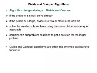
Divide-and conquer is a general algorithm design paradigm: Divide: divide the input data S in two or more disjoint subsets S1, S2, … Recur: solve the subproblems recursively Conquer: combine the solutions for S1,S2, …, into a solution for S The base case for the recursion are subproblems of constant size Analysis can be done using recurrence equations Divide-and-Conquer Divide-and-Conquer
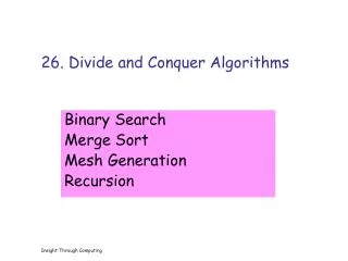
Divide-and-Conquer Examples • Finding maximums • Sorting: mergesort and quicksort • Binary tree traversals • Binary search • Multiplication of large integers • Matrix multiplication: Strassen’s algorithm • Convex-hull algorithms
A simple example • finding the maximum of a set S of n numbers
Time complexity • Time complexity: • Calculation of T(n): Assume n = 2k, T(n) = 2T(n/2)+1 = 2(2T(n/4)+1)+1 = 4T(n/4)+2+1 : =2k-1T(2)+2k-2+…+4+2+1 =2k-1+2k-2+…+4+2+1 =2k-1 = n-1
General Time complexity Dived & Conquer • Time complexity: or where S(n) : time for splitting M(n) : time for merging k : a constant c : a constant
Multiplication of Large Integers Consider the problem of multiplying two (large) n-digit integers represented by arrays of their digits such as:A = 12345678901357986429 B = 87654321284820912836The grade-school algorithm: a1 a2 … anb1 b2 … bn(d10)d11d12 … d1n (d20)d21d22 … d2n … … … … … … … (dn0)dn1dn2 … dnn Efficiency: Θ(n2) single-digit multiplications
First Divide-and-Conquer Algorithm A small example: A B where A = 2135 and B = 4014 A = (21·102 + 35), B = (40 ·102 + 14) So, A B = (21 ·102 + 35) (40 ·102 + 14) = 21 40 ·104 + (21 14 + 35 40) ·102 + 35 14 In general, if A = A1A2 and B = B1B2 (where A and B are n-digit, A1, A2, B1,B2 are n/2-digit numbers), A B = A1 B1·10n+ (A1 B2 + A2 B1) ·10n/2 + A2 B2 Recurrence for the number of one-digit multiplications M(n): M(n) = 4M(n/2), M(1) = 1Solution: M(n) = n2
Second Divide-and-Conquer Algorithm A B = A1 B1·10n+ (A1 B2 + A2 B1) ·10n/2 + A2 B2 The idea is to decrease the number of multiplications from 4 to 3: (A1 + A2 ) (B1 + B2 ) = A1 B1 + (A1 B2 + A2 B1) + A2 B2,I.e., (A1 B2 + A2 B1) = (A1 + A2 ) (B1 + B2 ) - A1 B1 - A2 B2,which requires only 3 multiplications at the expense of (4-1) extra add/sub. Recurrence for the number of multiplications M(n): M(n) = 3M(n/2), M(1) = 1 Solution: M(n) = 3log 2n= nlog 23 ≈n1.585
Example of Large-Integer Multiplication 2135 4014 = (21*10^2 + 35) * (40*10^2 + 14) = (21*40)*10^4 + c1*10^2 + 35*14 where c1 = (21+35)*(40+14) - 21*40 - 35*14, and 21*40 = (2*10 + 1) * (4*10 + 0) = (2*4)*10^2 + c2*10 + 1*0 where c2 = (2+1)*(4+0) - 2*4 - 1*0, etc. This process requires 9 digit multiplications as opposed to 16.
Conventional Matrix Multiplication • Brute-force algorithm • c00 c01 a00 a01 b00 b01 • = * • c10 c11 a10 a11 b10 b11 • a00 * b00 + a01 * b10 a00 * b01 + a01 * b11 • = • a10 * b00 + a11 * b10 a10 * b01 + a11 * b11 8 multiplications Efficiency class in general: (n3) 4 additions
Strassen’s Matrix Multiplication • Strassen’s algorithm for two 2x2 matrices (1969): • c00 c01 a00 a01 b00 b01 • = * • c10 c11 a10 a11 b10 b11 • m1 + m4 - m5 + m7 m3 + m5 • = • m2 + m4 m1 + m3 - m2 + m6 • m1 = (a00 + a11) * (b00 + b11) • m2 = (a10 + a11) * b00 • m3 = a00 * (b01 - b11) • m4 = a11 * (b10 - b00) • m5 = (a00 + a01) * b11 • m6 = (a10 - a00) * (b00 + b01) • m7 = (a01 - a11) * (b10 + b11) 7 multiplications 18 additions
Strassen’s Matrix Multiplication Strassen observed [1969] that the product of two matrices can be computed in general as follows: • C00 C01 A00 A01 B00 B01 • = * • C10 C11 A10 A11 B10 B11 • M1 + M4 - M5 + M7 M3 + M5 • = • M2 + M4 M1 + M3 - M2 + M6
Formulas for Strassen’s Algorithm M1 = (A00 + A11) (B00 + B11) M2 = (A10 + A11) B00 M3 = A00 (B01 - B11) M4 = A11 (B10 - B00) M5 = (A00 + A01) B11 M6 = (A10 - A00) (B00 + B01) M7 = (A01 - A11) (B10 + B11)
Analysis of Strassen’s Algorithm If n is not a power of 2, matrices can be padded with zeros. Number of multiplications: M(n) = 7M(n/2), M(1) = 1 Solution: M(n) = 7log 2n= nlog 27 ≈n2.807 vs. n3 of brute-force alg. Algorithms with better asymptotic efficiency are known but they are even more complex and not used in practice.
Mergesort • Split array A[0..n-1] into about equal halves and make copies of each half in arrays B and C • Sort arrays B and C recursively • Merge sorted arrays B and C into array A as follows: • Repeat the following until no elements remain in one of the arrays: • compare the first elements in the remaining unprocessed portions of the arrays • copy the smaller of the two into A, while incrementing the index indicating the unprocessed portion of that array • Once all elements in one of the arrays are processed, copy the remaining unprocessed elements from the other array into A.
Pseudocode of Merge Time complexity: Θ(p+q)= Θ(n) comparisons
Mergesort Example The non-recursive version of Mergesort starts from merging single elements into sorted pairs.
Analysis of Mergesort T(n) = 2T(n/2) + Θ(n), T(1) = 0 • All cases have same efficiency: Θ(n log n) of comparisons in the worst case is close to theoretical minimum for comparison-based sorting: • Space requirement: Θ(n) (not in-place) • Can be implemented without recursion (bottom-up)
p A[i]p A[i]p Quicksort • Select a pivot (partitioning element) – here, the first element • Rearrange the list so that all the elements in the first s positions are smaller than or equal to the pivot and all the elements in the remaining n-s positions are larger than or equal to the pivot (see next slide for an algorithm) • Exchange the pivot with the last element in the first (i.e., )subarray — the pivot is now in its final position • Sort the two subarraysrecursively
Partitioning Algorithm Time complexity: Θ(l-r) comparisons
Quicksort Example 5 3 1 9 8 2 4 7 2 3 1 4 5 8 9 7 1 2 3 4 5 7 8 9 1 23 4 57 8 9 1 2 3 4 5 7 8 9 1 2 3 4 5 7 8 9
Analysis of Quicksort • Best case: split in the middle — Θ(n log n) • Worst case: sorted array! — Θ(n2) • Average case: random arrays —Θ(n log n) • Improvements: • better pivot selection: median of three partitioning • switch to insertion sort on small subfiles • elimination of recursion These combine to 20-25% improvement • Considered the method of choice for internal sorting of large files (n≥ 10000) T(n) = T(n-1) + Θ(n)
Binary Search Very efficient algorithm for searching in sorted array: search K in A[0] . . . A[m] . . . A[n-1] If K = A[m], stop (successful search); otherwise, continue searching by the same method in A[0..m-1] if K < A[m] and in A[m+1..n-1] if K > A[m] l 0; r n-1 while l r do m (l+r)/2 if K = A[m] return m else if K < A[m] r m-1 else l m+1 return -1
Analysis of Binary Search • Time efficiency • worst-case recurrence: Tw (n) = 1 + Tw( n/2 ), Tw (1) = 1 solution: Tw(n) =log2(n+1)This is VERY fast: e.g., Tw(106) = 20 • Optimal for searching a sorted array • Limitations: must be a sorted array (not linked list) • Bad example of divide-and-conquer: because only one of the sub-instances is solved
Binary Tree Algorithms Binary tree is a divide-and-conquer ready structure! Ex. 1: Classic traversals (preorder, inorder, postorder) Algorithm Inorder(T) if T a a Inorder(Tleft)b c b c print(root of T)d e d e Inorder(Tright) Efficiency:Θ(n). Why? Each node is visited/printed once.
Binary Tree Algorithms (cont.) Ex. 2: Computing the height of a binary tree h(T) = max{h(TL), h(TR)} + 1 if T and h() = -1 Efficiency: Θ(n). Why?
Convex Hull • Convex hull: smallest convex set that includes given points. (Finding Extreme Points) Algorithm • P is extreme: if P is not in the all possible triangle • All possible triangles with n points: ɵ(n3) • For n points: ɵ(n4) P P2 P1
Convex Hull • Determinant det(A) = a11*det(A11)-a12*det(A12)+…+(-1)n-1 a1n*det(A1n)+ • P3 is in the left side of P1P2, if P2P1P3 angle <= 180o or P2 P1 P3
Graham’s Scan Algorithm • It is not a D&C algorithm • Select p with lowest Y from n points • Sort n points based on their angle with x coordinate. • While there is more points • IF angle of three sequential points (p1p2p3) < 180, • Else: remove p2 and p1 goes one back • T(n) = Sort+ Scan + angle check • T(n) = O(n lgn) + O(n) + O(1) = O(n lgn) Algorithms Design, Recurrences
Quickhull Algorithm Assume points are sorted by x-coordinate values 1- Identify extreme pointsP1 and P2(leftmost and rightmost) 2- Compute upper hull recursively: • find point Pmax that is farthest away from line P1P2 • compute the upper hull of the points to the left of line P1Pmax • compute the upper hull of the points to the left of line PmaxP2 3- Compute lower hull in a similar manner Pmax P2 P1
Efficiency of Quickhull Algorithm • Finding point farthest away from line P1P2 can be done in linear time • Time efficiency: T(n) = T(x) + T(y) + T(z) + T(v) + O(n), where x + y + z +v <= n. • worst case: Θ(n2) T(n) = T(n-1) + O(n) • average case: Θ(n log n) (under reasonable assumptions about distribution of points given) • If points are initially sorted by x-coordinate value, this can be accomplished in average by Θ(n) time and overall : Θ(n) + Θ(n log n) (sorting time) = Θ(n log n) • Several O(n log n) algorithms for convex hull are known