Download
1 / 10
100 likes | 279 Views
SECTION 4 RESPONSE METHOD. RESPONSE TYPES. The two types of response analysis in Linear Dynamics are: Transient Analysis (response through time) Frequency Response Analysis (response across a frequency range)

E N D
SECTION 4 RESPONSE METHOD
RESPONSE TYPES • The two types of response analysis in Linear Dynamics are: • Transient Analysis (response through time) • Frequency Response Analysis (response across a frequency range) • Transient analysis is intuitively the dynamic response we think of in many typical situations – impulsive loadings on a satellite during launch, response of an automobile to pot holes, earthquake response in a building. • An alternative is to vary the loading as a function of Frequency – this can simulate a shaker table or exciter where the input frequency is controlled and the response across a frequency range is investigated. u(t) P(t) t (secs) t (secs) Output Input u(f) P(f) F (Hz) Input Output F (Hz)
k k k M M 1 2 3 4 DOF: SPRING MASS SYSTEM • Look at the simple spring mass system from the previous section on normal modes • Run this model as a transient analysis and as a frequency response analysis for an overview of the two methods. • It was previously found that the natural frequencies and eigenvectors are:
k k M TRANSIENT ANALYSIS • In the first case, load grid point 3 with a force which varies sinusoidal with a magnitude of 1.0 at a frequency of .896 Hz (i.e. an input equal to the first resonant frequency) • In the second case, load the same point with another unit loading, but with a frequency of 1.731 Hz (i.e. an input equal to the second resonant frequency) • Damping in both cases is 2% critical Case 1 P(t)=1.0 sin 5.629 t Case 2 P(t)=1.0 sin 10.875 t P(t)
TRANSIENT ANALYSIS (Cont.) • For the first case, notice it takes around 33 secs of load input for the input load to reach an energy level where it balances the energy loss due to damping. • From this point on the response is steady state and we can see the amplitude of the two grid points 2 and 3 as +/- .015 and +/- .011 units.
TRANSIENT ANALYSIS (Cont.) • In the second case, notice a similar response, taking around 15 secs of load input for the input load to reach an energy level where it balances the energy loss due to damping • From this point on the response is steady state and we can see the amplitude of the two grid points 2 and 3 as +/- .0012 and +/- .003 units.
TRANSIENT ANALYSIS (Cont.) • The two sets of responses can be plotted as amplitude versus the driving frequency of loaded grid point: • The main response of the structure at the two natural frequencies has been convered, but it may be important to know what happens below .896 Hz, above 1.731 Hz and between the values • It is possible to do more transient analyses …. • Or a frequency response analysis can be used as shown. Grid 3 displacement Grid 2 Grid 2 Grid 3 frequency 1.731 .896
FREQUENCY RESPONSE ANALYSIS • The Frequency Response analysis: • inputs the loading as a continuous function of frequency • calculates the response of the two grid points as a function of frequency at defined frequency response points • The displacement values from the Transient Response analysis match those of the Frequency Response analysis F1 = 0.896 Hz U2 = 0.011 U3 = 0.015 F2 = 1.731 Hz U2 = 0.003 U3 = 0.001 Node 3 Node 2
RESPONSE TYPES • It may be that one or other type of loading is defined in a specification and it may be required to carry out the respective response analysis • However, both types of response may be useful in assessing a structure under a loading environment • For a transient analysis, it is necessary to assess the frequency content of the response, either by simple methods such as peak to peak estimate of the time period, or carrying out a Fourier analysis • Whichever technique is used it is essential that the normal modes of the structure have been investigated first. This is a theme that will be discussed in later case studies and workshops.
MODAL AND DIRECT METHODS • In the previous section it was seen that a response through time can be defined in the physical coordinate system x(t) or in terms of the modal coordinate system • It was also seen that the number of modal coordinates needed to define a response is typically a small fraction of the number of physical coordinates • This motivates us to have an option to solve dynamics problems in the modal coordinate system in the interests of saving CPU time • Extend the technique to responses as a function of frequency • Thus MSC.Marc linear transient dynamic solutions have two versions. • Direct - The solution is solved in terms of physical coordinates. • Modal - The solution is solved in terms of modal coordinates • The steps in the modal solution sequences are: • Transform from physical to modal coordinates. • Solve in modal coordinates • Transform back to physical coordinates