Topic
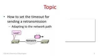
Topic. How to set the timeout for sending a retransmission A dapting to the network path. Lost?. Network. Retransmissions. With sliding window, the strategy for detecting loss is the timeout Set timer when a segment is sent Cancel timer when ack is received

Topic
E N D
Presentation Transcript
Topic • How to set the timeout for sending a retransmission • Adapting to the network path Lost? Network CSE 461 University of Washington
Retransmissions • With sliding window, the strategy for detecting loss is the timeout • Set timer when a segment is sent • Cancel timer when ack is received • If timer fires, retransmit data as lost Retransmit! CSE 461 University of Washington
Timeout Problem • Timeout should be “just right” • Too long wastes network capacity • Too short leads to spurious resends • But what is “just right”? • Easy to set on a LAN (Link) • Short, fixed, predictable RTT • Hard on the Internet (Transport) • Wide range, variable RTT CSE 461 University of Washington
Example of RTTs BCNSEABCN Round Trip Time (ms) Seconds CSE 461 University of Washington
Example of RTTs (2) BCNSEABCN Variation due to queuing at routers, changes in network paths, etc. Round Trip Time (ms) Propagation (+transmission) delay ≈ 2D Seconds CSE 461 University of Washington
Example of RTTs (3) Timer too high! Need to adapt to the network conditions Round Trip Time (ms) Timer too low! Seconds CSE 461 University of Washington
Adaptive Timeout • Keep smoothed estimates of the RTT (1) and variance in RTT (2) • Update estimates with a moving average • SRTTN+1 = 0.9*SRTTN + 0.1*RTTN+1 • SvarN+1 = 0.9*SvarN + 0.1*|RTTN+1– SRTTN+1| • Set timeout to a multiple of estimates • To estimate the upper RTT in practice • TCP TimeoutN = SRTTN + 4*SvarN CSE 461 University of Washington
Example of Adaptive Timeout RTT (ms) SRTT Svar Seconds CSE 461 University of Washington
Example of Adaptive Timeout (2) Early timeout Timeout (SRTT + 4*Svar) RTT (ms) Seconds CSE 461 University of Washington
Adaptive Timeout (2) • Simple to compute, does a good job of tracking actual RTT • Little “headroom” to lower • Yet very few early timeouts • Turns out to be important for good performance and robustness CSE 461 University of Washington
Topic • How TCP works! • The transport protocol used for most content on the Internet We TCP/IP! We love TCP/IP! We love TCP/IP! We love TCP/IP! TCP TCP TCP Network CSE 461 University of Washington
TCP Features • A reliable bytestream service » • Based on connections • Sliding window for reliability » • With adaptive timeout • Flow control for slow receivers • Congestion control to allocate network bandwidth This time Next time CSE 461 University of Washington
Reliable Bytestream • Message boundaries not preserved from send() to recv() • But reliable and ordered (receive bytes in same order as sent) Sender Receiver Four segments, each with 512 bytes of data and carried in an IP packet 2048 bytes of data delivered to app in a single recv() call CSE 461 University of Washington
Reliable Bytestream (2) • Bidirectional data transfer • Control information (e.g., ack) piggybacks on data segments in reverse direction ackba ackab data ab data ba A B CSE 461 University of Washington
TCP Header (1) • Ports identify apps (socket API) • 16-bit identifiers CSE 461 University of Washington
TCP Header (2) • seq/ack used for sliding window • Selective Repeat, with byte positions CSE 461 University of Washington
TCP Sliding Window – Receiver • Cumulative ack tells next expected byte sequence number (“LAS+1”) • Optionally, selective acks (SACK) give hints for receiver buffer state • List up to 3 ranges of received bytes ack up to 100 and 200-299 CSE 461 University of Washington
TCP Sliding Window – Sender • Uses an adaptive retransmission timeout to resend data from LAS+1 • Uses heuristics to infer loss quickly and resend to avoid timeouts • “Three duplicate acks” treated as loss ack 100, 200-299 ack 100, 200-399 ack 100, 200-499 ack 100 Sender decides 100-199 is lost CSE 461 University of Washington
TCP Header (4) • Window size for flow control • Relative to ack, and in bytes CSE 461 University of Washington
Other TCP Details • Many, many quirks you can learn about its operation • But they are the details • Biggest remaining mystery is the workings of congestion control • We’ll tackle this next! CSE 461 University of Washington
Where we are in the Course • More fun in the Transport Layer! • The mystery of congestion control • Depends on the Network layer too Application Transport Network Link Physical CSE 461 University of Washington
Topic • Understanding congestion, a “traffic jam” in the network • Later we will learn how to control it What’s the hold up? Network CSE 461 University of Washington
Nature of Congestion • Routers/switches have internal buffering for contention Input Output . . . . . . . . . . . . Fabric Output Buffer Input Buffer CSE 461 University of Washington
Nature of Congestion (2) • Simplified view of per port output queues • Typically FIFO (First In First Out), discard when full Router Router = Queued Packets (FIFO) Queue CSE 461 University of Washington
Nature of Congestion (3) • Queues help by absorbing bursts when input > output rate • But if input > output rate persistently, queue will overflow • This is congestion • Congestion is a function of the traffic patterns – can occur even if every link have the same capacity CSE 461 University of Washington
Effects of Congestion • What happens to performance as we increase the load? CSE 461 University of Washington
Effects of Congestion (2) • What happens to performance as we increase the load? CSE 461 University of Washington
Effects of Congestion (3) • As offered load rises, congestion occurs as queues begin to fill: • Delay and loss rise sharply with more load • Throughput falls below load (due to loss) • Goodput may fall below throughput (due to spurious retransmissions) • None of the above is good! • Want to operate network just before the onset of congestion CSE 461 University of Washington
Bandwidth Allocation • Important task for network is to allocate its capacity to senders • Good allocation is efficient and fair • Efficient means most capacity is used but there is no congestion • Fair means every sender gets a reasonable share the network CSE 461 University of Washington
Bandwidth Allocation (2) • Key observation: • In an effective solution, Transport and Network layers must work together • Network layer witnesses congestion • Only it can provide direct feedback • Transport layer causes congestion • Only it can reduce offered load CSE 461 University of Washington
Bandwidth Allocation (3) • Why is it hard? (Just split equally!) • Number of senders and their offered load is constantly changing • Senders may lack capacity in different parts of the network • Network is distributed; no single party has an overall picture of its state CSE 461 University of Washington
Bandwidth Allocation (4) • Solution context: • Senders adapt concurrently based on their own view of the network • Design this adaption so the network usage as a whole is efficient and fair • Adaption is continuous since offered loads continue to change over time CSE 461 University of Washington
Topic • What’s a “fair” bandwidth allocation? • The max-min fair allocation CSE 461 University of Washington
Recall • We want a good bandwidth allocation to be fair and efficient • Now we learn what fair means • Caveat: in practice, efficiency is more important than fairness CSE 461 University of Washington
Efficiency vs. Fairness • Cannot always have both! • Example network with traffic AB, BC and AC • How much traffic can we carry? B A C 1 1 CSE 461 University of Washington
Efficiency vs. Fairness (2) • If we care about fairness: • Give equal bandwidth to each flow • AB: ½ unit, BC: ½, and AC, ½ • Total traffic carried is 1 ½ units B A C 1 1 CSE 461 University of Washington
Efficiency vs. Fairness (3) • If we care about efficiency: • Maximize total traffic in network • AB: 1 unit, BC: 1, and AC, 0 • Total traffic rises to 2 units! B A C 1 1 CSE 461 University of Washington
The Slippery Notion of Fairness • Why is “equal per flow” fair anyway? • AC uses more network resources (two links) than AB or BC • Host A sends two flows, B sends one • Not productive to seek exact fairness • More important to avoid starvation • “Equal per flow” is good enough CSE 461 University of Washington
Generalizing “Equal per Flow” • Bottleneck for a flow of traffic is the link that limits its bandwidth • Where congestion occurs for the flow • For AC, link A–B is the bottleneck B A C 10 1 Bottleneck CSE 461 University of Washington
Generalizing “Equal per Flow” (2) • Flows may have different bottlenecks • For AC, link A–B is the bottleneck • For BC, link B–C is the bottleneck • Can no longer divide links equally … B A C 10 1 CSE 461 University of Washington
Max-Min Fairness • Intuitively, flows bottlenecked on a link get an equal share of that link • Max-min fair allocation is one that: • Increasing the rate of one flow will decrease the rate of a smaller flow • This “maximizes the minimum” flow CSE 461 University of Washington
Max-Min Fairness (2) • To find it given a network, imagine “pouring water into the network” • Start with all flows at rate 0 • Increase the flows until there is a new bottleneck in the network • Hold fixed the rate of the flows that are bottlenecked • Go to step 2 for any remaining flows CSE 461 University of Washington
Max-Min Example • Example: network with 4 flows, links equal bandwidth • What is the max-min fair allocation? CSE 461 University of Washington
Max-Min Example (2) • When rate=1/3, flows B, C, and D bottleneck R4—R5 • Fix B, C, and D, continue to increase A Bottleneck CSE 461 University of Washington
Max-Min Example (3) • When rate=2/3, flow A bottlenecks R2—R3. Done. Bottleneck Bottleneck CSE 461 University of Washington
Max-Min Example (4) • End with A=2/3, B, C, D=1/3, and R2—R3, R4—R5 full • Other links have extra capacity that can’t be used • , linksxample: network with 4 flows, links equal bandwidth • What is the max-min fair allocation? CSE 461 University of Washington
Adapting over Time • Allocation changes as flows start and stop Time CSE 461 University of Washington
Adapting over Time (2) Flow 1 slows when Flow 2 starts Flow 1 speeds up when Flow 2 stops Flow 3 limit is elsewhere Time CSE 461 University of Washington