Data Mining: Data
Data Mining: Data. Lecture Notes for Chapter 2 Introduction to Data Mining by Tan, Steinbach, Kumar. What is Data?. Collection of data objects and their attributes An attribute is a property or characteristic of an object Examples: eye color of a person, temperature, etc.

Data Mining: Data
E N D
Presentation Transcript
Data Mining: Data Lecture Notes for Chapter 2 Introduction to Data Mining by Tan, Steinbach, Kumar
What is Data? • Collection of data objects and their attributes • An attribute is a property or characteristic of an object • Examples: eye color of a person, temperature, etc. • Attribute is also known as variable, field, characteristic, or feature • A collection of attributes describe an object • Object is also known as record, point, case, sample, entity, or instance Attributes Objects
Data • The Type of Data • The Quality of the Data • Preprocessing steps to make the data more suitable for data mining • Analyzing data in terms of relationships • Example 2.1
Attribute Values • Attribute values are numbers or symbols assigned to an attribute • Distinction between attributes and attribute values • Same attribute can be mapped to different attribute values • Example: height can be measured in feet or meters • Different attributes can be mapped to the same set of values • Example: Attribute values for ID and age are integers • But properties of attribute values can be different • ID has no limit but age has a maximum and minimum value
Measurement of Length • The way you measure an attribute is somewhat may not match the attributes properties.
Types of Attributes • There are different types of attributes • Nominal • Examples: ID numbers, eye color, zip codes • Ordinal • Examples: rankings (e.g., taste of potato chips on a scale from 1-10), grades, height in {tall, medium, short} • Interval • Examples: calendar dates, temperatures in Celsius or Fahrenheit. • Ratio • Examples: temperature in Kelvin, length, time, counts
Properties of Attribute Values • The type of an attribute depends on which of the following properties it possesses: • Distinctness: = • Order: < > • Addition: + - • Multiplication: * / • Nominal attribute: distinctness • Ordinal attribute: distinctness & order • Interval attribute: distinctness, order & addition • Ratio attribute: all 4 properties
Attribute Type Description Examples Operations Nominal The values of a nominal attribute are just different names, i.e., nominal attributes provide only enough information to distinguish one object from another. (=, ) zip codes, employee ID numbers, eye color, sex: {male, female} mode, entropy, contingency correlation, 2 test Ordinal The values of an ordinal attribute provide enough information to order objects. (<, >) hardness of minerals, {good, better, best}, grades, street numbers median, percentiles, rank correlation, run tests, sign tests Interval For interval attributes, the differences between values are meaningful, i.e., a unit of measurement exists. (+, - ) calendar dates, temperature in Celsius or Fahrenheit mean, standard deviation, Pearson's correlation, t and F tests Ratio For ratio variables, both differences and ratios are meaningful. (*, /) temperature in Kelvin, monetary quantities, counts, age, mass, length, electrical current geometric mean, harmonic mean, percent variation
Attribute Level Transformation Comments Nominal Any permutation of values If all employee ID numbers were reassigned, would it make any difference? Ordinal An order preserving change of values, i.e., new_value = f(old_value) where f is a monotonic function. An attribute encompassing the notion of good, better best can be represented equally well by the values {1, 2, 3} or by { 0.5, 1, 10}. Interval new_value =a * old_value + b where a and b are constants Thus, the Fahrenheit and Celsius temperature scales differ in terms of where their zero value is and the size of a unit (degree). Ratio new_value = a * old_value Length can be measured in meters or feet.
Discrete and Continuous Attributes • Discrete Attribute • Has only a finite or countably infinite set of values • Examples: zip codes, counts, or the set of words in a collection of documents • Often represented as integer variables. • Note: binary attributes are a special case of discrete attributes • Continuous Attribute • Has real numbers as attribute values • Examples: temperature, height, or weight. • Practically, real values can only be measured and represented using a finite number of digits. • Continuous attributes are typically represented as floating-point variables.
Asymmetric Attributes • Only presence – a non-zero attribute value is regarded as important • Student’s record indicating whether he/she has taken a course or not • Are students more similar in the number of courses they have taken or those they haven’t? • Asymmetric Binary attributes – non-zero values are important - associative analysis
Types of data sets • Record • Data Matrix • Document Data • Transaction Data • Graph • World Wide Web • Molecular Structures • Ordered • Spatial Data • Temporal Data • Sequential Data • Genetic Sequence Data
Important Characteristics of Structured Data • Dimensionality • Curse of Dimensionality • Sparsity (affects data with asymmetric features) • Only presence counts • May work very well in data mining as 1’s are important • Resolution • Patterns depend on the scale • Properties are different at different resolutions, surface of the Earth at different resolutions
Record Data • Data that consists of a collection of records, each of which consists of a fixed set of attributes • Usually stored in flat files or relational databases • No explicit relationship among records or data fields
Data Matrix (Pattern matrix) • If data objects have the same fixed set of numeric attributes, then the data objects can be thought of as points in a multi-dimensional space, where each dimension represents a distinct attribute • Such data set can be represented by an m by n matrix, where there are m rows, one for each object, and n columns, one for each attribute
Document Data (ex of Sparse Data Matrix) • Each document becomes a `term' vector, • each term is a component (attribute) of the vector, • the value of each component is the number of times the corresponding term occurs in the document. Non-zero = important?
Transaction Data (Market basket data) • A special type of record data, where • each record (transaction) involves a set of items. • For example, consider a grocery store. The set of products purchased by a customer during one shopping trip constitute a transaction, while the individual products that were purchased are the items.
Graph Data • Examples: Generic graph and HTML Links • The graph captures relationships among data objects • The data objects themselves are represented as graphs
Graph Data • Data with relationships among Objects • The relationships among objects frequently convey important information • Often data objects are mapped to nodes of the graph • Data with Objects that are Graphs • When objects have structures – the objects contain subobjects that have relationships, ex. A chemical component.
Chemical Data • Benzene Molecule: C6H6 • Makes it possible to: • determine which substructures occurs frequently in a set of compounds • whether the presence of any of these substructures is associated with the presence or absence of certain chemical properties (melting point, etc) H C
Ordered Data Attributes have relationships that involve order in time or space • Sequences of transactions (temporal data) Items/Events An element of the sequence
Sequence Data • What is the difference between sequential data and sequence data?
Ordered Data • Genomic sequence data
Ordered Data • Spatio-Temporal Data Average Monthly Temperature of land and ocean Spatial auto-correlation - Objects that are physically close tend to be similar in other ways as well. Example: two points that are close to each other have similar rainfall.
Time Series Data • A series of measurements taken over time How do we handle non-record data?
Data Quality • What kinds of data quality problems? • How can we detect problems with the data? • What can we do about these problems? • Detection and correction • Use of algorithms that can tolerate poor quality • Examples of data quality problems: • Noise and outliers • missing values • duplicate data
Precision, Bias, and Accuracy • Precision – The closeness of repeated measurements to one another • Bias – A systematic variation of measurements from the quantity being measured • Accuracy – The closeness of measurements to the true value of the quantity being measured
Noise and artifacts (distortion or addition) • Noise refers to modification of original values • Examples: distortion of a person’s voice when talking on a poor phone and “snow” on television screen Two Sine Waves Two Sine Waves + Noise
Outliers • Outliers are data objects with characteristics that are considerably different than most of the other data objects in the data set
Missing Values • Reasons for missing values • Information is not collected (e.g., people decline to give their age and weight) • Attributes may not be applicable to all cases (e.g., annual income is not applicable to children) • Handling missing values • Eliminate Data Objects • Estimate Missing Values • Ignore the Missing Value During Analysis • Replace with all possible values (weighted by their probabilities)
Missing Values • How do we estimate Missing Values? Example: 2 5 11 .?. 47 • How do we replace with all possible values (weighted by their probabilities) Suppose domain was [0—15} imagine a 4-bit image Example: 2 3 4 2 8 ? 2 3 2 3 4 Think PDF, Think CDF
Duplicate Data • Data set may include data objects that are duplicates, or almost duplicates of one another • Major issue when merging data from heterogeneous sources • Examples: • Same person with multiple email addresses • Data cleaning • Process of dealing with duplicate data issues
Application Related Issues Quote: “Data is of high quality if it is suitable for its intended use” • Timeliness • Data start to age as soon as it is collected .. Ex. Data collected on people who are buying Pentium II’s • Relevance • The available data must contain the information necessary for the application .. Ex. Insurance data without age and gender • Sampling bias .. Ex. surveys • Knowledge about the data • Quality of documentation .. Missing value issue
Data Preprocessing Some of the most important ideas: • Aggregation • Sampling • Dimensionality Reduction • Feature subset selection • Feature creation • Discretization and Binarization • Attribute Transformation These fall into two categories: selecting data objects and attributes for analysis or creating/changing the attributes. Improving: Time Cost, and Quality
Aggregation (less is more) • Combining two or more attributes (or objects) into a single attribute (or object) • How would you deal with the quantitative attributes? Sum, avg • How would you deal with the qualitative attributes? Omitted or summarized as a set • Purpose (commonly used in OLAP) • Data reduction • Reduce the number of attributes or objects less memory, fast, allow more expensive algorithm • Change of scale • Cities aggregated into regions, states, countries, etc • More “stable” data • Aggregated data tends to have less variability
Aggregation Variation of Precipitation in Australia Standard Deviation of Average Monthly Precipitation Standard Deviation of Average Yearly Precipitation
Sampling • Sampling is the main technique employed for data selection. • It is often used for both the preliminary investigation of the data and the final data analysis. • Statisticians sample because obtaining the entire set of data of interest is too expensive or time consuming. • Sampling is used in data mining because processing the entire set of data of interest is too expensive or time consuming. With reduced data, i.e., better and more expensive algorithms can be used
Sampling … • The key principle for effective sampling is the following: • using a sample will work almost as well as using the entire data sets, if the sample is representative • A sample is representative if it has approximately the same property (of interest) as the original set of data
Types of Sampling • Simple Random Sampling • There is an equal probability of selecting any particular item • Sampling without replacement • As each item is selected, it is removed from the population • Sampling with replacement • Objects are not removed from the population as they are selected for the sample. • In sampling with replacement, the same object can be picked up more than once • Stratified sampling • Split the data into several partitions; then draw random samples from each partition
Sample Size 8000 points 2000 Points 500 Points
Sample Size • What sample size is necessary to get at least one object from each of 10 groups.
Progressive Sampling • Start with a small sample, and then increase the sample size until a sample of sufficient size is obtained. Problem – Need a mechanism to determine whether the sample size is large enough
Curse of Dimensionality • When dimensionality increases, data becomes increasingly sparse in the space that it occupies • Definitions of density and distance between points, which is critical for clustering and outlier detection, become less meaningful • Randomly generate 500 points • Compute difference between max and min distance between any pair of points
Dimensionality Reduction • Purpose: • Avoid curse of dimensionality • Reduce amount of time and memory required by data mining algorithms • Allow data to be more easily visualized • May help to eliminate irrelevant features or reduce noise • Techniques • Principle Component Analysis (PCA) • Singular Value Decomposition (SVD) also related to PCA • Others: supervised and non-linear techniques
Dimensionality Reduction: PCA • Goal is to find a projection that captures the largest amount of variation in data x2 e x1 Principal components: 1) Linear combination of original attributes, 2) are orthogonal (perpendicular) to each other, and 3) capture the maximum amount of variation in the data.
Dimensionality Reduction: PCA • Find the eigenvectors of the covariance matrix • The eigenvectors define the new space x2 e x1
Dimensionality Reduction: ISOMAP • Construct a neighbourhood graph • For each pair of points in the graph, compute the shortest path distances – geodesic distances By: Tenenbaum, de Silva, Langford (2000)
Feature Subset Selection • Another way to reduce dimensionality of data • Redundant features • duplicate much or all of the information contained in one or more other attributes • Example: purchase price of a product and the amount of sales tax paid • Irrelevant features • contain no information that is useful for the data mining task at hand • Example: students' ID is often irrelevant to the task of predicting students' GPA