Download

1 / 38
390 likes | 582 Views
Fundamental Lower Bound for Node Buffer Size in Intermittently Connected Wireless Networks. Yuanzhong Xu, Xinbing Wang Shanghai Jiao Tong University , China. Outline. Introduction Motivations Objectives Model and Assumption Percolation of Active Nodes Lower Bound In Supercritical Case

E N D
Fundamental Lower Bound for Node Buffer Size inIntermittently Connected Wireless Networks Yuanzhong Xu, Xinbing Wang Shanghai Jiao Tong University, China
Outline Introduction Motivations Objectives Model and Assumption Percolation of Active Nodes Lower Bound In Supercritical Case Lower Bound In Subcritical Case Discussion on Length of Time Slot Conclusion Buffer in Intermittently Connected Network Presentation 2
Motivation • Under certain constraints, wireless networks are • Only intermittently connectivity: • A complete path from the source to the destination does not exist all the time. • Example: • Wireless sensor networks: Node sleeping mode for energy saving. ([7, Dousse]) • CR networks: Secondary users wait for availability of wireless channel. ([8, Ren & Zhao]) • Mobile networks:Nodes move out of reach. ([9, Kong & Yeh]) Buffer in Intermittently Connected Network Presentation 3
Motivation • Intermittently connectivity requires adequate node buffer, even with infinite channel capacity and processing speed, • Temporarily store the packets not ready to be sent out. Buffer in Intermittently Connected Network Presentation 4
Objectives • We focus on node buffer occupation in static random wireless networks with intermittent connectivity due to node inactivity: • How does the minimum buffer requirement for each node increase as the network size grows? • What is the achievable lower bound for node buffer size? Buffer in Intermittently Connected Network Presentation 5
Outline Introduction Model and Assumption Percolation of Active Nodes Lower Bound In Supercritical Case Lower Bound In Subcritical Case Discussion on Length of Time Slot Conclusion Buffer in Intermittently Connected Network Presentation 6
Model and Assumption – I/V • Node Locations: • First consider a Poisson point process on R2 with density λ • Locations of nodes are points within the region: • Direct Links: • Each node covers a disk shaped area with radius ½ • Two nodes have a direct link if and only if they overlap: Buffer in Intermittently Connected Network Presentation 7
Model and Assumption – II/V • Assumption on Node Density: • There exists an infinite connected cluster in R2(giant cluster) • Nodes in giant cluster: connected nodes • Number of connected nodes is proportional to n • Larger density => larger connected proportion: Buffer in Intermittently Connected Network Presentation 8
Model and Assumption – III/V • Node inactivity – Each node switch between active state and inactive state: • Time is slotted, slot length: • States of each active nodes are i.i.d. among time slots. • The probability to be inactive is for all nodes. • States of different nodes are i.i.d. • Model Notation: Buffer in Intermittently Connected Network Presentation 9
Model and Assumption – IV/V • Traffic Pattern of Connected Nodes – Random Unicast • Permanent source-destination pairs (connected). • Each source messages to destination in constant rate . • Transmission in multi-hop. • Buffering • In each hop, if the transmitter or the receiver is inactive, the messages should be buffered in the transmitter until both are active. Buffer in Intermittently Connected Network Presentation 10
Model and Assumption – V/V • Assumption on Capacity and Processing speed • Channel capacity is large enough to be viewed as infinity, compared to the actual utilization. • Node processing speed is also infinite, compared to the state-switching frequency. • Message slot • Messages generated by u during time slot t whose destination is v have the same route, and exist in the same node at the end of a time slot. Denoted by . • Size of one message slot: Buffer in Intermittently Connected Network Presentation 11
Outline Introduction Model and Assumption Percolation of Active Nodes Lower Bound In Supercritical Case Lower Bound In Subcritical Case Discussion on Length of Time Slot Conclusion Buffer in Intermittently Connected Network Presentation 12
Percolation of Active Nodes • Active nodes density: • Threshold for probability of inactivity: • Supercritical Case: • active giant exists in each time slot • Subcritical Case: • no active giant in each time slot Buffer in Intermittently Connected Network Presentation 13
Outline Introduction Model and Assumption Percolation of Active Nodes Lower Bound In Supercritical Case Lower Bound In Subcritical Case Discussion on Length of Time Slot Conclusion Buffer in Intermittently Connected Network Presentation 14
Lower Bound In Supercritical Case – I/VII • Supercritical case:Achievable Lower bound – Constant Order: • For a connected node in with , at time slot , • Lower bound at least needs to buffer messages generating by itself when it is inactive. • achievable ? Buffer occupation in w at time slot t Buffer in Intermittently Connected Network Presentation 15
Lower Bound In Supercritical Case – II/VII • Achievable with Optimal Routing Scheme (ORS) • 3 stages of ORS in (for source and destination ) : • Stage 1 – Source relay & bufferingRelay along a linear pathNodes keep a copy until one node in the path belongs to active giant. (source buffering path – nodes thathave received the message); • Stage 2 – Transmit via active giant • Stage 3 – Destination relay Buffer in Intermittently Connected Network Presentation 16
Lower Bound In Supercritical Case – III/VII • Achievable with Optimal Routing Scheme (ORS) • 3 stages of ORS in (for source and destination ) : • Stage 1 – Source relay & buffering • Stage 2 – Transmit via active giantTransmit from the source buffering path to the nearest node a f to destination. (without latency) • Stage 3 – Destination relay Buffer in Intermittently Connected Network Presentation 17
Lower Bound In Supercritical Case – IV/VII • Achievable with Optimal Routing Scheme (ORS) • 3 stages of ORS in (for source and destination ) : • Stage 1 – Source relay & buffering • Stage 2 – Transmit via active giant • Stage 3 – Destination relayAlong the shortest path from todestination.(destination buffering path) Buffer in Intermittently Connected Network Presentation 18
Lower Bound In Supercritical Case – V/VII • Why finite buffer in ORS? • Active giant spreads all over the network: • Only considering active giant in one time slot – Vacant components are small. • [17] • In Stage I, • buffering path is circulated bya vacant component. • Small source buffering path • (finite expectation of size) Buffer in Intermittently Connected Network Presentation 19
Lower Bound In Supercritical Case – VI/VII • Why finite buffer in ORS? • Active giant spreads all over the network: • Only considering active giant in one time slot – Vacant components are small. • [17] • In Stage III, destination is circulated by a vacant component with size at least the distance between and destination Small destination buffering path • (finite expectation of size) Buffer in Intermittently Connected Network Presentation 20
Lower Bound In Supercritical Case – VII/VII • Why finite buffer in ORS? • Finite-sized source buffering path and destination buffering path • Finite Latency; One node only buffers messages with near sources or destinations. • Finite buffer occupation in ORS. Buffer in Intermittently Connected Network Presentation 21
Outline Introduction Model and Assumption Percolation of Active Nodes Lower Bound In Supercritical Case Lower Bound In Subcritical Case Discussion on Length of Time Slot Conclusion Buffer in Intermittently Connected Network Presentation 22
Lower Bound In Subcritical Case – I/III • Lower bound: • The smallest latency of a message slot for u to v satisfies: • By Little’s Law, average buffer occupation among all connected nodes : • – The lower bound is . Buffer in Intermittently Connected Network Presentation 23
Lower Bound In Subcritical Case – II/III • Achievability • Assuming transmission path from to is along the straight line connecting them: • Hop by hop transmission, path between neighboring flag nodes is the shortest one. • In this scheme, lower bound is achieved. Buffer in Intermittently Connected Network Presentation 24
Lower Bound In Subcritical Case – III/III • Proof Sketch of Achievability • Giant component (including both active and inactive nodes) • If belongs to the path from to ( ), then it cannot be far from the line connecting them ( ) • Prove that serves for S-D pairs • lower bound is achieved. Buffer in Intermittently Connected Network Presentation 25
Outline Introduction Model and Assumption Percolation of Active Nodes Lower Bound In Supercritical Case Lower Bound In Subcritical Case Discussion on Length of Time Slot Conclusion Buffer in Intermittently Connected Network Presentation 26
Discussion on Length of Time Slot • In both supercritical and subcritical cases, lower bounds for buffer occupation scales linearly to the length of time slot. • With constant probability of node inactivity, • smaller results in smaller buffer requirements. • When , it is equivalent to no inactivity but channel capacity decreases to , similar to TDMA. Buffer in Intermittently Connected Network Presentation 27
Outline Introduction Model and Assumption Percolation of Active Nodes Lower Bound In Supercritical Case Lower Bound In Subcritical Case Discussionon Length of Time Slot Conclusion Buffer in Intermittently Connected Network Presentation 28
Conclusion • We study the lower bounds for node buffer in intermittently connected network. • In supercritical case, the achievable lower bound does not increase as the network size grows. • In subcritical case, the achievable lower bound is . • In both cases, lower bounds for buffer occupation scales linearly to the length of time slot. Buffer in Intermittently Connected Network Presentation 29
Reference Buffer in Intermittently Connected Network Presentation 31
Reference Buffer in Intermittently Connected Network Presentation 32
Reference Buffer in Intermittently Connected Network Presentation 33
Intermittently Connected Long Path • A path of n nodes • With finite channel capacity,assume every node send all messages in its buffer to the next node: • Buffer occupation of nodes on the path has large variance in time domain. Buffer in Intermittently Connected Network Presentation 34
Intermittently Connected Long Path • With finite channel capacity,assume every node send all messages in its buffer to the next node: Buffer in Intermittently Connected Network Presentation 35
Intermittently Connected Long Path • Non-empty ratio: the proportion of time slots during which buffer is empty. Buffer in Intermittently Connected Network Presentation 36
Intermittently Connected Long Path • Improvement by a simple mechanism –Restrict the maximum amount of messages sent in one time slot of each hop. p = 0.5, in one time slot each hop can transmit at most 30 message slots. Buffer in Intermittently Connected Network Presentation 37
Intermittently Connected Long Path • Improvement by a simple mechanism –Restrict the maximum amount of messages sent in one time slot of each hop. p = 0.5, in one time slot each hop can transmit at most 30 message slots. Buffer in Intermittently Connected Network Presentation 38