Download
1 / 30
300 likes | 333 Views
This presentation discusses the types of wildland fires, the game method model, the WRF-Fire model, and how the two models can work together. Future work plans will also be presented.

E N D
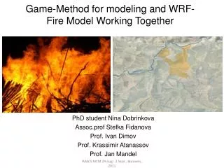
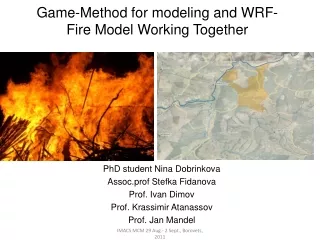
Game-Method for modeling and WRF-Fire Model Working Together PhD student Nina Dobrinkova Assoc.prof Stefka Fidanova Prof. Ivan Dimov Prof. Krassimir Atanassov Prof. Jan Mandel IMACS MCM 29 Aug.- 2 Sept., Borovets, 2011
In this presentation: • Will be presented the types of wildland fires • Will be presented basics of game-method model and some results • Will be presented WRF-Fire model and some results • Will be presented a conception about how the two models can work together • Future work plans IMACS MCM 29 Aug.- 2 Sept., Borovets, 2011
Types of wildland fires Surface fireshave rate of spread of the forest fire advancing in burning materials like grass, shrubs, small trees. These fires are the most common in nature. Crown firesare the combustion of tree crowns that overlie the surface fire and surface fuels. They are very intensive in burning and hard to fight with. Spotting firesrefer to new ignitions ahead of the main fire front started by firebrands lofted by the fire and transported by the wind. Spotting can advance fire over barriers many kilometers away from the current fire perimeter and alter fire growth patterns and behavior. Fire accelerationis defined as the rate of increase in spread rate for a given ignition source that all fire environmental conditions remain constant. IMACS MCM 29 Aug.- 2 Sept., Borovets, 2011
Forest fire statistics in South european countries • 1971 to 2006 • considerable increase of the number of fires after 1990 (more than 1000 in year 2000) • more than 30 times increase of the burned area in the recent years The number of fires since 1980 according to statistics done for the southern member states has increased rapidly in the last few years IMACS MCM 29 Aug.- 2 Sept., Borovets, 2011
Forest fire statistics - Bulgaria Bulgaria’s statistic about forest fires 1994 to 2010 Natura 2000 zones in 2007 There is significant overlapping of the protected zones and the one which fires has occurred in the last 16 years IMACS MCM 29 Aug.- 2 Sept., Borovets, 2011
Game-Method Model for Filed Fires L=A(K)=A1(A1(…A1(K)…)) Where: A1 - is the transition rule K – initial configuration L – final configuration IMACS MCM 29 Aug.- 2 Sept., Borovets, 2011
Experimental results (1) Our test area is divided on N x M bins. We fill on random principle the bins with numbers from 0 to 9, which would be our burning coefficients. We do correctness check by averaging every bin with respect to all simulated tests. The equation used was: We do the same with averaging action with the burned area: IMACS MCM 29 Aug.- 2 Sept., Borovets, 2011
Experimental results (2) • We prepare a small example with 9 x 9 bins just to show how the fire is dispersed. This is the initial area, where the 0 are non burning material, and the other coefficients are potential fire beds.
WRF-Fire basics (1) Mathematically the fire model is posed in the horizontal (x,y) plane. The fire propagation is in semi-empirical approach and it is assumed that the fire spreads in the direction normal to the fireline. This is given from the the modified Rothermel’s formula: S=min{B0,R0 + ɸW + ɸS}, where B0 is the spread rate against the wind; R0 is the spread rate in the absence of wind; ɸW is the wind correction ɸS is the terrain correction IMACS MCM 29 Aug.- 2 Sept., Borovets, 2011
WRF-Fire basics (2) Once the fuel is ignited, the amount of the fuel at location (x, y) is given by: Where : t is the time; ti is the ignition time; F0 is the initial amount of fuel; T is the time for the fuel to burn down to 1/e of the original quantity IMACS MCM 29 Aug.- 2 Sept., Borovets, 2011
WRF-Fire basics (3) From slides (1) and (2) we have idea about the plane, where the fire will spread and the fuel which we want to ignited, but we also need the heat flux, which is inserted as the time derivative of the temperature, while the latent heat flux as the time derivative of water vapor concentration. This scheme is required because atmospheric models with explicit time stepping, such as WRF, do not support flux boundary conditions. IMACS MCM 29 Aug.- 2 Sept., Borovets, 2011
WRF-Fire basics (4) From the previous three slides we have the plane of the fire, the ignited fuel, the heat flux, but we also will need the burning region at time t. It is represented by level set function ɸ, as the set of all points (x, y) where ɸ (x, y, t) < 0. The level set function satisfies a partial differential equation for dynamic implicit surfaces: Where is the Eucledian norm of the gradient of ɸ. IMACS MCM 29 Aug.- 2 Sept., Borovets, 2011
Simulation results (1) • The objective of this third simulation is to present the simulation capabilities of WRF-Fire model with real input data. • Atmospheric model was run on 2 domains with 250m and 50m resolution • 41 vertical levels were used • The fire module, coupled with the atmosperic domain is run on 5m resolution with 0.3s time step • Simulated burned area and actual data from the Ministry of Agriculture, Forest and Food showed good comparison IMACS MCM 29 Aug.- 2 Sept., Borovets, 2011
Parallel performance • Computations were performed on the Janus cluster at the University of Colorado. The computer consists of nodes with dual Intel X5660 processors (total 12 cores per node), connected by QDR InfiniBand • The model runs as fast as real time on 120 cores and it is twice faster on 360 (real time coef. = 0.99) IMACS MCM 29 Aug.- 2 Sept., Borovets, 2011
Simulation results (2) IMACS MCM 29 Aug.- 2 Sept., Borovets, 2011
Simulation results (3) • the heat flux (red is high) • burned area (black) • atmospheric flow(purple is over 10m/s) • Note the updraft caused by the fire • Ground image from Google Earth IMACS MCM 29 Aug.- 2 Sept., Borovets, 2011
Combining the two methods together • From the meteorological point of view wind is the most important parameter for the fire spread. It is missing from the game-method model and is included in the simulations of WRF-Fire. That is why we decided to combine both models and include wind in the game-method model. This can be done in two ways: • With average wind value, which does not correspond to the real wind behavior • -With random field describing the wind, where we will use Monte Carlo simulation. We define Z(x), x ∈ R2 to be random field and we have: • Fx1,x2,…,xn (X1,X2, ..., Xn) = P (z1 ≤ X1,X2, ...,zn ≤ Xn) • for z1 = Z (x1) and n can be any integer. IMACS MCM 29 Aug.- 2 Sept., Borovets, 2011
Sub-cases • The representation of the random field of the wind we divide in two sub-cases: • -The wind direction and velocity are having random behavior (hard for computational estimations) • -The wind has fixed direction and random speed velocity • We set width of the random field parameter – w • In cases: • Small values of width w – the wind parameter will have speed in small interval close to the case the velocity is fixed • Relatively big random field of the wind with different in range values, which is because of the non constant behavior of the wind, where we can calibrate the model with the meteorological conditions IMACS MCM 29 Aug.- 2 Sept., Borovets, 2011
Future work In the described steps with conditions for the random field of the wind Monte Carlo methods can be used for simulation results and tests. We will focus on comprising between exact rotational-wind estimator (in its two-dimensional version) and approximate estimator The proposed scheme represents two and three –dimensional turbolence over discretized spatial domains. We propose combination between game method for modelling and the meteorology from WRF-Fire method. The will be simulated by random field and Monte Carlo methods. Our future work will be focused on learning the random field parameters in various range for w. We will test with sensitivity analysis the influence of the value of this parameter on the models output. We will compare the results with cases of fixed velocity. IMACS MCM 29 Aug.- 2 Sept., Borovets, 2011
Thank you for your attention! Nina Dobrinkova Institute of Information and Comunication Technologies - Bulgarian Academy of Sciences,nido@math.bas.bg IMACS MCM 29 Aug.- 2 Sept., Borovets, 2011