The Estimation Problem
Understand the process of transitioning states, estimating parameters from data through maximum likelihood, and avoiding overfitting with examples. Learn the importance of likelihood function and how MLE seeks the best parameters.

The Estimation Problem
E N D
Presentation Transcript
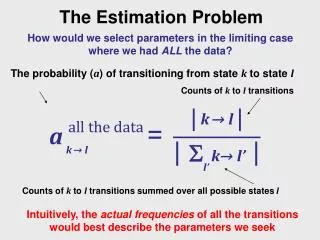
The probability (a) of transitioning from state k to state l The Estimation Problem How would we select parameters in the limiting case where we had ALL the data? Counts of k to l transitions k→ l Counts of k to l transitions summed over all possible states l Sl’ k→ l’ k→ l Intuitively, the actual frequencies of all the transitions would best describe the parameters we seek
The Estimation Problem What about when we only have a sample? Consider: X = “S--+++” Before we collected the data, the probability of this sequence is a function of , our set of unknown parameters: P(X|) = P(“S--+++”|) P(X|) = as→-a-→-a-→+a+→+a+→+ However, our data is fixed. We have already collected it. The parameters are also fixed, but unknown. We can therefore imagine values for the parameters, and treat the probability of the observed data as a function of
The Estimation Problem The Likelihood Function When we treat the probability of the observed data as a function of the parameters, we call this the likelihood function L(|X) = P(“S--+++”|) L(|X)= as→-a-→-a-→+a+→+a+→+ • A few things to notice: • The probability of any particular sample we get is generally going to be pretty low regardless of the true values of • The likelihood here still tells us some valuable information! We know, for instance that a-→+is not zero, etc. Caution! The likelihood function does not define a probability distribution or density and it does not encompass an area of 1
Maximum Likelihood Estimation Maximum Likelihood Estimation seeks the solution that “best” explains the observed dataset 𝜃ML= argmaxP(X|𝜃) = argmaxlogP(X|𝜃) Or Translation: “select as our maximum likelihood parameters those parameters that resulted in a maximization of the probability of the observation given those parameters”. i.e. we seek to maximize P(X|𝜃)over all possible 𝜃 This is sometimes called the maximum likelihood criterion
Maximum Likelihood Estimation Log likelihood is often very handy as we often would otherwise need to deal with a long product of terms… 𝜃ML= 𝑎𝑟𝑔𝑚𝑎𝑥 log P(xi|𝜃) P k i=1 = 𝑎𝑟𝑔𝑚𝑎𝑥 log P(xi|𝜃) S k i=1 This often comes about because there are multiple outcomes that need to be considered
Maximum Likelihood Estimation Sometimes proving some parameter choice maximizes the likelihood function is the “tricky bit” In general case, this is often done by finding the zeros of the derivative of the likelihood function, or by some other trick such as forcing the function into some particular form and relying on an inequality to prove it must be maximum Let’s skip the gory details, and try to motivate this intuitively…
The Estimation Problem Maybe it’s enough to convince ourselves that… k→ l will approach….. Sl’ k→ l’ k→ l P(k→l|𝜃All the data) as the amount of sample data increases to the limit where we finally have all the data…. Let’s see how this plays out with a simple simulation…
Maximum Likelihood Estimation Typical plot of single sample of 10 nucleotides MLE is prone to overfitting the data in the case where the sample is small The underlying distribution this was sampled from was uniform (pA = 0.25,pC= 0.25,pG= 0.25,pT= 0.25)
Maximum Likelihood Estimation Typical plot of 10 samples of 10 nucleotides The underlying distribution this was sampled from was uniform (pA = 0.25,pC= 0.25,pG= 0.25,pT= 0.25)
Maximum Likelihood Estimation Typical plot of 100 samples of 10 nucleotides The underlying distribution this was sampled from was uniform (pA = 0.25,pC= 0.25,pG= 0.25,pT= 0.25)
Maximum Likelihood Estimation Typical plot of 1000 samples of 10 nucleotides The underlying distribution this was sampled from was uniform (pA = 0.25,pC= 0.25,pG= 0.25,pT= 0.25)