Download
1 / 51
510 likes | 539 Views
Learn about the fundamentals of data representation through maps, classification techniques, and visual resources. This comprehensive guide covers various types of maps, scaling methods, symbology, and normalization techniques essential for effective data communication.

E N D
Data Representation and Mapping Ming-Chun Lee
What is a map? • A miniaturized and convenient representation of spatial reality • A picture or diagram, usually two-dimensional, showing all or part of the Earth and is a device for transferring selected information about the mapped area to the map viewer
Types of Maps • Reference Maps - Used to emphasize the location of spatial phenomenon • USGS topographic maps • Road maps • Thematic maps - used to display the spatial pattern of a particular theme • Maps of population in the United States • Geological maps
Characteristics of Maps • All maps are reductions of reality • All maps portray data which has been generalized, classified, and simplified • All maps use symbols to designate elements of reality. Data are portrayed by the use of various marks, such as dots, lines, patterns, and colors which are referred in a legend
Data classification and scaling • Nominal Scaling Data are differentiated by qualitative or intrinsic differences between features, without a quantitative relationship. The nominal scale locates and names items and places them in exclusive categories. • Ordinal Scaling The data are ranked based on some quantitative measurement. They are only ranked from lowest to highest, without defining their numerical value. • Interval/Ratio Scaling Scaling adds the dimension of distance between the ranked data by employing some standard units. Scaling adds magnitude to the ranks. Interval scaling starts at some arbitrary point, such as 32°F, Ratio scaling begins with zero.
The range of visual resources • As cartographers reduce the world to points, lines, and areas, they use a variety of visual resources. Jacques Bertin in his book The Semiology of Graphics (1983), inventories these resources using the categories of size, shape, value, texture or pattern, hue, orientation, and shape.
To increase the legibility of figures, use different line types and colors (and labels) rather than just different colors
Qualitative: nominal classes Dr. Cynthia Brewer / Department of Geography / The Pennsylvania State University
Sequential: for numeric classes Dr. Cynthia Brewer / Department of Geography / The Pennsylvania State University
Qualitative sequential: numeric and nominal Dr. Cynthia Brewer / Department of Geography / The Pennsylvania State University
colors are nice, but what’s wrong with this map? Primary home heating fuel. U.S. Department of Commerce
Vector Symbology:Discrete Attribute Data • Single Symbol • All Features Look the Same • Categories • Unique Values • Using One Attribute, Set a Distinct Symbol for Each Value • Unique Values, Many Fields • Using Several Attributes, Set a Distinct Symbol for Each Combination • Match to Symbols In a Style • Use Preset Symbology Based on an Attribute
Vector Symbology:Discrete Attribute Data Unique Values:Arterial Class Unique Values, Many Fields:Arterial Class & Bike Class Single Symbol
Vector Symbology: Continuous Attribute Data • Quantities • Graduated Colors • Maps Colors Along a Gradient to Discrete, Ordered Ranges of Attribute Values • Graduated Symbols • Maps Sizes of Symbols to Discrete, Ordered Ranges of Attribute Values • Proportional Symbols • Continuously Varies Symbol Sizes by Attribute Values
Vector Symbology: Continuous Attribute Data GraduatedColors GraduatedSymbol Sizes ProportionalSymbol Sizes
Vector Symbology: Charts • Charts • Pie • Bar/Column • Stacked
Symbology:Raster Layers Views of Radio Towers • Unique Values • Discrete Data Discrete Colors • Classified • Continuous Data Discrete Colors • Stretched • Continuous Data Continuous Colors Aspect Slope
Map Layout:Data Frames Layout View Toolbar Data Frame Object Extents of GIS Data Data Frame Edge Paper Margin Paper Edge
Map Layout:Full Map Layout Title North Arrow Scale Body Landmark Text (opt.) Legend Overview (opt.)
Normalization • Set Value to One Attribute • Set Normalization to Another Attribute • ArcMap Calculates Color Based On: • Displayed Value = Value / Normalization • Examples: • Density: Value / Area • Proportional Growth: New Value / Old Value • Proportional Population:Subgroup Population / Total Population
Classification • How are Continuous Data Categorized in Symbology? • Classification Methods • Equal Interval/Defined Interval • Place Breaks at Equal Intervals, Specifying Number or Width of Breaks • Standard Deviation • Place Breaks at Equal Standard Deviations From the Mean Value • Quantile • Place Breaks Such That Groups Have Equal Size Memberships • Natural Breaks • Place Breaks Between Clusters of Data • Manual Breaks
Histogram • x-Axis: • The full range of data values, classified into narrow range categories • y-Axis: • Number of features/cells, or frequency • Bars: • The number of features in each narrow range category
Equal Interval/Defined Interval • Guarantees a linear relationship between the data values and the color selected
Standard Deviation • Similar to Equal Interval, but uses a statistical basis for determining the interval size
Quantile • Guarantees that each color will be assigned to approximately the same number of features • Effectively divides your data into equally-sized groups • Results in Greatest Overall Differentiation
Natural Breaks • Uses an algorithm to place breaks such that: • The variance within groups is minimized, and • The variance between groups is maximized • Results will tend to be irregularly-sized intervals • This is the default in ArcMap
Manual Breaks • Can reflect policy-based or arbitrary thresholds and categories • Tedious to set up