Estimation Techniques for Dose-Response Functions

1. Estimation Techniques for Dose-response Functions Presented by Bahman Shafii, Ph.D. Statistical Programs College of Agricultural and Life Sciences University of Idaho

2. Acknowledgments • Research partially funded by USDA-ARS Hatch Project • IDA01412,Idaho Agricultural Experiment Station. • Collaborators: • William J. Price Ph. D., Statistical Programs, • University of Idaho. • Steven Seefeldt, Ph. D., USDA -ARS, • University of Alaska Fairbanks.

3. Introduction • Dose-response models are common in agricultural research. • They can encompass many types of problems: • Modeling environmental effects due to exposure to chemical or temperature regimes. • Estimation of time dependent responses such as germination, emergence, or hatching. • (e.g. Shafii and Price 2001; Shafii, et al. 2009) • Bioassay assessments via calibration curves and quantal estimation. (e.g. Shafii and Price 2006)

4. Estimation • Curve estimation. • Linear or non-linear techniques. • Estimate other quantities: • percentiles. • typically: LD50, LC50, EC50, etc. • percentile estimation problematic. • inverted solutions. • unknown distributions. • approximate variances.

5. The response distribution: • Continuous • Normal • Log Normal • Gamma, etc. • Discrete - quantal responses • Binomial, Multinomial (yes/no) • Poisson (count)

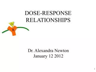
6. Dose • The response form: • Typically expressed as a nonlinear curve • increasing or decreasing sigmoidal form • increasing or decreasing asymptotic form Response Dose

7. Bioassay and Calibration • Given a dose-response curve and an observed • response: • What dose generated the response? • What is the probability of a dose given an • observed response and the calibration curve? • This problem fits naturally into a Bayesian framework.

8. Response Dose Measured Response Unknown Dose

9. Typical dose-response estimation assumes that the • functional form or tolerance distribution, • is known, e.g. a sigmoidal shape. • In some cases, however, it may be advantageous to • relax this assumption and restrict estimation • to a family of dose-response forms. • The dose-response population consists of a • mixture of subpopulations which can not be • sampled separately. • The dose-response series exhibits a more complex • behavior than a simple sigmoidal shape, • e.g. hormesis.

10. Objectives • Outline estimation methods for dose- • response models. • Traditional approaches. • Probit - Least Squares. • Modern approaches. • Probit - Maximum Likelihood • Generalized non-linear models. • Bayesian solutions.

11. Objectives • Demonstrate solutions for calibration of an unknown dose with a binary response • assuming: • A known dose-response form. • Standard MLE estimation. • Standard Parametric Bayesian estimation. • A family of dose-response forms. • Nonparametric Bayesian estimation.

12. Estimation Methods • where • pij = yij / N and yij is the number of successes out of N • trials in the jth replication of the ith dose. • b0 and b1 are regression parameters and ei is a random • error; eij ~ N(0,s2). • Minimize: SSerror =  (pij - probit)2 ^ • Traditional Approach • Probit Analysis - Least Squares • A linearized least squares estimation (Bliss, 1934 ; Fisher, 1935; • Finney, 1971): • Probiti = F -1(pij) = b0 + b1*dosei + eij (1)

13.   •  is a convenient CDF form or “tolerance • distribution“, e.g. • Normal:pij = (1/2) exp((x-)2/2 • Logistic:pij = 1 / (1 + exp( -b1( dosei - b0 )) • Modified Logistic: pij = C + (C-M) / (1 + exp( -b1(dosei -b0)) • (e.g. Seefeldt et al. 1995) • Gompertz: pij = b0 (1 - exp(exp(-b1(dose)))) • Exponential:pij = b0 exp(-b1(dose)) • SAS: PROC REG.

14. Modern Approaches • Probit Analysis -Maximum Likelihood • The responses, yij, are assumed binomial at each dose i • with parameter pi. Using the joint likelihood, L(pi) : • Maximize: L(pi) P (pi)yij (1 - pi)(N - yij) (2) • for data set yij where pi = F (b0 + b1*dosei ) and b0, b1, • and dosei are those given previously. • The CDF, F, is typically defined as a Normal, Logistic, or • Gompertz distribution as given above. • SAS: PROC PROBIT.

15. Probit Analysis • Limitations: • Least squares limited. • Linearized solution to a non-linear problem. • Even under ML, solution for percentiles approximated. • inversion. • use of the ratio b0/b1 (Fieller, 1944). • Appropriate only for proportional data. • Assumes the response F-1(pij) ~ N(m, s2). • Interval estimation and comparison of percentile • values approximated.

16. Modern Approaches (cont) • Nonlinear Regression - IterativeLeast Squares • Directly models the response as: • yij = f(dosei) + eij(3) • where yij is an observed continuous response, f(dosei) • may be generalized to any continuous function of dose • and eij ~ N(0, s2). • Minimize: SSerror =  [ yij - f(dosei) ]2. • SAS: PROC NLIN.

17. Nonlinear Regression - Iterative Least Squares • Limitations: • assumes the data, yij, is continuous; could be discrete. • the response distribution may not be Normal, • i.e.eij ~ N(0, s2). • standard errors and inference are asymptotic. • treatment comparisons difficult in PROC NLIN. • differential sums of squares, or • specialized SAS codes ; PROC IML.

18. Modern Approaches (cont) • Generalized Nonlinear Model - Maximum Likelihood • Directly models the response as: • yij = f(dosei) + eij • where yij and f(dosei) are as defined above. • Estimation through maximum likelihood where the • response distribution may take on many forms: • Normal: yij ~ N(i, ) , • Binomial: yij ~ bin(N, pi) , • Poisson: yij ~ poisson(i) , or • in general: yij ~ ƒ().

19. Generalized Nonlinear Model - Maximum Likelihood • Maximize: L() Pƒ( | yij) (4) • Nonlinear estimation. • Response distribution not restricted to Normal. • May also incorporate random components into the model. • Treatment comparisons easier in SAS. • Contrast and estimate statements. • SAS: PROC NLMIXED.

20. Generalized Nonlinear Model - Inference • Formulate a full dummy variable model encompassing k • treatments. • The joint likelihood over the k treatments becomes: • L(k) Pijkƒ(k | yijk) (5) • where yijk is the jth replication of the ith dose in the kth • treatment and qk are the parameters of the kth treatment. • Comparison of parameter values is then possible through • single and multiple degree of freedom contrasts.

21. Generalized Nonlinear Model • Limitations • percentile solution may still be based on inversion or • Fieller’s theorem. • inferences based on normal theory approximations. • standard errors and confidence intervals asymptotic.

22. Modern Approaches (cont) • Bayesian Estimation - Iterative Numerical Techniques • Considers the probability of the parameters, q, • given the data yij. • Using Bayes theorem, estimate: • p(q|yij) = p(yij|q)*p(q) (6) • p(yij|q)*p(q)dq where p(q|yij) is the posterior distribution of q given the data yij, p(yij|q) is the likelihood defined above, and p(q) is a prior probability distribution for the parameters q.

23. Bayesian Estimation - Iterative Numerical Techniques • Nonlinear estimation. • Percentiles can be found from the distribution of q. • The likelihood is same as Generalized Nonlinear Model. • flexibility in the response distribution. • f(dosei) any continuous function of dose. • Inherently allows updating of the estimation. • Correct interval estimation (credible intervals). • agrees well with GNLM at midrange percentiles. • can perform better at extreme percentiles. • SAS: PROC MCMC.

24. Bayesian Estimation - Iterative Numerical Techniques • Limitations • User must specify a prior probability p(q). • Estimation requires custom programming. • SAS: PROC MCMC • Specialized software: WinBUGS • Computationally intensive solutions. • Requires statistical expertise. • Sample programs and data are available at: • http://www.uidaho.edu/ag/statprog

25. Calibration Methods • Tolerance Distribution: Logistic • The response yij/Ni at dose i = 1 to k, and replication • j=1 to r , is binomial with the proportion of success • given by: • yij/Ni = M/(1 + exp(-b (dosei - g))) (7) • where b is a rate related parameter and g is the • dosei for which the proportion of success, • yij/Ni , is M/2. M is the theoretical maximum • proportion attainable.

26. A convenient generalization of (1) will allow g to • represent any dose at which yij/Ni = Q: yij/Ni = M*C / (C + exp(-b (dosei - g))) (8) Where the constant C = Q/(M – Q). Note that, if Q = M/2, then C = 1 and equation (8) reverts to the standard form given in (7). Equation (8), therefore, permits an unknown dose at a given response, Q, to be estimated through parameter g.

27. Maximum Likelihood • Given the binomial responses, yij/Ni, a joint • likelihood may be defined as: • L(pi | yij/Ni) Pij (pi)yij (1 - pi)(Ni - yij) (9) • Where the binomial parameter ,pi , is defined by (8) • and the associated parameters, q = [M, b, g], are • estimated through maximization of (9). Ni and yij • are the total number of trials and number of • successes, respectively. • Inferences on g are carried out assuming g ~ N(mg, sg). • SAS: PROC NLMIXED

28. Bayesian: Parametric • A Bayesian posterior distribution for q is given by: • pr(q| yij/Ni) pr(yij/Ni |q) · pr(q) (10) • where pr(yij/Ni j|q) is the likelihood shown in (9) and pr(q) • is a prior distribution for the parameters q = [M, b, g]. Estimation of q is carried out through numerically intensive techniques such as MCMC. (e.g. Price and Shafii 2005) • Inference on g is obtained through integration of (10) over the parameter space of M and b.

29. Bayesian: Nonparametric • This methodology was first proposed by Mukhopadhyay (2000) and • followed by Kottas et al. (2002). • The technique considers the dose-response series as a • multinomial process with parameters P = [p1, p2, p3, … pk]. • Assuming the responses, yij/Ni, are binomial, a likelihood can • then be defined as: • L(P| yij/Ni) Pij (pi)yij (1 - pi)(Ni - yij) (11)

30. If the random segments between true response rates, pi , • are distributed as a Dirichlet Process (DP), a joint prior • distribution on the pi may then be defined by: • pr(P) Pi(pi – pi - 1)(li - 1) (12) • where li = a{ F0(dose i) – F0(dose i – 1 ) }, a is a precision • parameter , and F0 is a base tolerance distribution. • The precision parameter, a, reflects how closely the final estimation follows the base distribution. Low values indicate less correspondence , while larger values indicate a tighter association. • The base distribution, F0(.), defines a family of tolerance distributions.

31. A posterior distribution for P can then be defined by • combining (11) and (12) as: • pr(P | yij/Ni) Pij (pi)yij (1 - pi)(Ni - yij) Pi(pi – pi - 1)(li - 1) • (13) • Estimation of this posterior is again carried out numerically using techniques such as MCMC. • Inference on an unknown dose, g, at a known response p0 = y0/N0, is obtained through sampling of the posterior given in (13) .

32. Concluding Remarks • Dose-response models have wide application in agriculture. • They are useful for quantifying the relative efficacy of treatments. • Probit models of estimation are limited in scope. • Generalized nonlinear and Bayesian models provide the most • flexible framework for dose-response estimation. • Can use various response distributions • Can use various dose-response models. • Can incorporate random model effects. • Can be used to compare treatments. • GNLM: full dummy variable modeling. • Bayesian methods: probability statements. • Generalized nonlinear models sufficient in most • situations. • Bayesian estimation is preferred when estimating • extreme percentiles.

33. Concluding Remarks (cont) • Bioassay is an import part of dose-response analysis. • Determining an unknown dose can be problematic for • some parametric functional forms. • Dose estimation fits naturally in a Bayesian framework. • Methodology proposed here uses a base tolerance • distribution. • Should be used and interpreted with caution. • Standard model assessment techniques still apply. • Introduces more uncertainty into the estimation situation. • Some dose-response data may not follow typical • sigmoidal patterns.

34. References Bliss, C. I. 1934. The method of probits. Science, 79:2037, 38-39 Bliss, C. I. 1938. The determination of dosage-mortality curves from small numbers. Quart. J. Pharm., 11: 192-216. Berkson, J. 1944. Application of the Logistic function to bio-assay. J. Amer. Stat. Assoc. 39: 357-65. Feiller, E. C. 1944. A fundamental formula in the statistics of biological assay and some applications. Quart. J. Pharm. 17: 117-23. Finney, D. J. 1971. Probit Analysis. Cambridge University Press, London. Fisher, R. A. 1935. Appendix to Bliss, C. I.: The case of zero survivors., Ann. Appl. Biol., 22: 164-5. SAS Inst. Inc. 2004. SAS OnlineDoc, Version 9, Cary, NC. Seefeldt, S.S., J. E. Jensen, and P. Fuerst. 1995. Log-logistic analysis of herbicide dose-response relationships. Weed Technol. 9:218-227. Kottas, A., M. D. Branco, and A. E. Gelfand. 2002. A Nonparametric Bayesian Modeling Approach for Cytogenetic Dosimetry. Biometrics 58, 593-600.

35. References Mukhopadhyay, S. 2000. Bayesian Nonparametric Inference on the Dose Level with Specified Response Rate. Biometrics 56, 220-226. Price, W. J. and B. Shafii. 2005. Bayesian Analysis of Dose-response Calibration Curves. Proceedings of the Seventeenth Annual Kansas State University Conference on Applied Statistics in Agriculture [CDROM], April 25-27, 2005. Manhattan Kansas. Shafii, B. and W. J. Price. 2001. Estimation of cardinal temperatures in germination data analysis. Journal of Agricultural, Biological and Environmental Statistics. 6(3):356-366. Shafii, B. and W. J. Price. 2006. Bayesian approaches to dose-response calibration models. Abstract: Proceedings of the XXIII International Biometrics Conference [CDROM], July 16 - 21, 2006. Montreal, Quebec Canada. Shafii, B., Price, W.J., Barney, D.L. and Lopez, O.A. 2009. Effects of stratification and cold storage on the seed germination characteristics of cascade huckleberry and oval-leaved bilberry. Acta Hort. 810:599-608.

36. Questions / Comments