Lecture 18 Expectation Maximization
Lecture 18 Expectation Maximization . Machine Learning. Last Time. Expectation Maximization Gaussian Mixture Models. Term Project. Projects may use existing machine learning software weka , libsvm , liblinear , mallet, crf ++, etc. But must experiment with Type of data

Lecture 18 Expectation Maximization
E N D
Presentation Transcript
Lecture 18Expectation Maximization Machine Learning
Last Time • Expectation Maximization • Gaussian Mixture Models
Term Project • Projects may use existing machine learning software • weka, libsvm, liblinear, mallet, crf++, etc. • But must experiment with • Type of data • Feature Representations • a variety of training styles – amount of data, classifiers. • Evaluation
Gaussian Mixture Model • Mixture Models. • How can we combine many probability density functions to fit a more complicated distribution?
Gaussian Mixture Model • Fitting Multimodal Data • Clustering
Gaussian Mixture Model • Expectation Maximization. • E-step • Assign points. • M-step • Re-estimate model parameters.
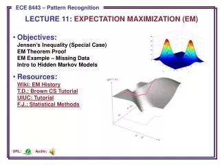
Today • EM Proof • Jensen’s Inequality • Clustering sequential data • EM over HMMs
How can we be sure GMM/EM works? • We’ve already seen that there are multiple clustering solutions for the same data. • Non-convex optimization problem • Can we prove that we’re approaching some maximum, even if many exist.
Bound maximization • Since we can’t optimize the GMM parameters directly, maybe we can find the maximum of a lower bound. • Technically: optimize a convex lower bound of the initial non-convex function.
EM as a bound maximization problem • Need to define a function Q(x,Θ) such that • Q(x,Θ) ≤ l(x,Θ) for all x,Θ • Q(x,Θ) = l(x,Θ) at a single point • Q(x,Θ) is concave
EM as bound maximization • Claim: • for GMM likelihood • The GMM MLE estimate is a convex lower bound
EM Correctness Proof • Prove that l(x,Θ) ≥ Q(x,Θ) Likelihood function Introduce hidden variable (mixtures in GMM) A fixed value of θt Jensen’s Inequality (coming soon…)
EM Correctness Proof GMM Maximum Likelihood Estimation
The missing link: Jensen’s Inequality • If f is concave (or convex down): • Incredibly important tool for dealing with mixture models. if f(x) = log(x)
Generalizing EM from GMM • Notice, the EM optimization proof never introduced the exact form of the GMM • Only the introduction of a hidden variable, z. • Thus, we can generalize the form of EM to broader types of latent variable models
General form of EM • Given a joint distribution over observed and latent variables: • Want to maximize: • Initialize parameters • E Step: Evaluate: • M-Step: Re-estimate parameters (based on expectation of complete-data log likelihood) • Check for convergence of params or likelihood
Applying EM to Graphical Models • Now we have a general form for learning parameters for latent variables. • Take a Guess • Expectation: Evaluate likelihood • Maximization: Reestimate parameters • Check for convergence
Clustering over sequential data • HMMs • What if you believe the data is sequential, but you can’t observe the state.
Training latent variables in Graphical Models • Now consider a general Graphical Model with latent variables.
EM on Latent Variable Models • Guess • Easy, just assign random values to parameters • E-Step: Evaluate likelihood. • We can use JTA to evaluate the likelihood. • And marginalize expected parameter values • M-Step: Re-estimate parameters. • Based on the form of the models generate new expected parameters • (CPTs or parameters of continuous distributions) • Depending on the topology this can be slow