Download

1 / 68
690 likes | 936 Views
Experimental and theoretical methods to study protein folding. Experiments. Thermal denaturation Chemical denaturation Mechanical unfolding Kinetic experiments Mutational studies. Techniques. Differential scanning calorimetry (DSC) Spectroscopy Circular dichroism (CD) Fluorescence

E N D
Experimental and theoreticalmethods to study protein folding
Experiments • Thermal denaturation • Chemical denaturation • Mechanical unfolding • Kinetic experiments • Mutational studies
Techniques • Differential scanning calorimetry (DSC) • Spectroscopy • Circular dichroism (CD) • Fluorescence • Nuclear magnetic resonance (NMR) • Small angle X-ray (SAXS) and small angle neutron scattering (SANS) • Atomic force microscopy (AFM)
Wild type Acid-denaturatedwildtype L16A mutant C-terminal peptide Religa et al., J. Mol. Biol., 333, 977-991 (2003)
F-values Mutation affects the folded state but not the transition state Mutation affects both the folded state and the transition state Matouschek A, Kellis JT, Serrano L, Fersht AR. (1989). Mapping the transition state and pathway of protein folding by protein engineering. Nature 340:122
Structure of closed and open form of theDnaK (Hsp70) chaperone
Fluorescencestudies of closing and opening of Hsp70 Mapa et al., Molecular Cell 38, 89, 2010.
Theoretical studies of protein structure and protein folding • Need to express energy of a system as function of coordinates • Need an algorithm to explore the conformational space
Partition of the energy of interactions with respect to topological distance 1,4-nonbonded interactions Eel+Enb Bonding interactions, Es only Torsional interactions Etor 1,3-interactions Eb only 1,5-interactions Eel+EVdW
Bond distortion energy Es(d) d d0 d
Comparison of the actual bond-energy curve with that of the harmonic approximation
Potentials that take into account the asymmetry of bond-energy curve Anharmonic potential Morse potential Harmonic potential Anharmonic potential Morse potential E [kcal/mol] d [A]
Energy of bond-angle distortion Eb(q) q kq q0 q
Basic types of torsional potentials Single bond between sp3carbons or between sp3 carbon and nitrogen Example: C-C-C-C quadruplet 60 50 40 30 20 10 0 Double or partially double bonds Example: C-C=C-C quadruplet Etor [kcal/mol] Single bond between electronegative atoms (oxygens, sulfurs, etc.). Example: C-S-S-C quadruplet dihedral angle [deg]
Nonbonded Lennard-Jones (6-12) potential Enb [kcal/mol] -e r0 s r [A]
Other nonbonded potentials Buckingham potential 10-12 potential used in some force fields (e.g., ECEPP) for proton…proton donor pairs
Solvent in simulations • Explicit water • TIP3P • TIP4P • TIP5P • SPC • Implicit water • Solvent accessible surface area (SASA) models • Molecular surface area models • Poisson-Boltzmann approach • Generalized Born surface area (GBSA) model • Polarizable continuum model (PCM)
0.00 e O 0.15 Å H H M 0.520 e -1.040 e -0.834 e O 0.9572 Å H H 104.52o 0.417 e TIP3P model TIP4P model sO=3.1535 Å eO=0.1550 kcal/mol sO=3.1507 Å eO=0.1521 kcal/mol
Solvent accessible surface area (SASA) models siFree energy of solvation of atomu iper unit area, Aisolvent accessible surface of atomi dostępna
Vila et al., Proteins: Structure, Function, and Genetics, 1991, 10, 199-218.
Comparison of the lowest-energy conformations of [Met5]enkefalin (H-Tyr-Gly-Gly-Phe-Met-OH) obtained with the ECEPP/3 force field in vacuo and with the SRFOPT model vacuum SRFOPT
Compariosn of the molecular sufraces of the lowest-energy conformation of [Met5]enkefaliny obtained without and with the SRFOPT model vacuum SRFOPT
Molecular surface are model sSurface tension Amolecular surface area
All-atom representation of polypeptide chains Coarse-grained representation of polypeptide chains
Coarse-grained force fields Physics-based potentials (statistical-mechanical formulation) X : primary variablespresent in the model Y : secondary variables not present in the model (solvent, side-chain dihedral angles, etc.) E(X,Y) : all-atom energy function. Statistical potentials X – geometric variables c – residue types s – sequence context
Leu-Leu pair A – radial correlation function B – reference distribution function C -
Searching the conformational space Low (Lowest)-energy conformations Canonical conformational ensembles Monte Carlo withminimization (MCM) Basinhopping Canonical MC Canonical MD Replica-exchange MC (REMC) Diffusionequationmethod (DEM Replica-exchange MD (REMD) Geneticalgorithms Simulatedannealing Moleculardynamics Local energy minimization Smoothing energy surface Monte Carlo
Local vs. global minimization f(x) Start Local minimum Global minimum x
General scheme of local minimization of multivariate functions: • Choose the initial approximation x(0). • In pth iteration, compute the search direction d(p). • Locate x(p+1) as a minimum on the serarch direction (minimization of a function in one variable). • Terminate when convergence has been achieved or maximum number of iterations exceeded. x2 x(0) f(x(p)+td(p)) x(2) x(1) d(2) x* d(1) a* a x1
Lowest-energy structureof gramicidinS computed with the ECEPP force field (M. Dygert, N. Go, H.A. Scheraga, Macromolecules, 8, 750-761 (1975). This structure turned out to be identical with the NMR structure determined later.
The C-terminal part of HDEA protein found by global minimization of the UNRES coarse-grained effective energy function. The N-terminal part of HDEA Liwo et al., PNAS, 96, 5482–5485 (1999)
Comparison of the experimental strucgture of bacteriocin AS-48 fromE. faecalis with the structure obtained by global minimization of the UNRES force field (Pillardy et al., Proc. Natl.Acad. Sci. USA., 98, 2329-2333 (2001))
“Potential energy” or “free energy”? Nature (and a canonical simulation) finds the basin with the lowest free energy, at a given temperature which might happen to but does not have to contain the conformation with the lowest potential energy. The global-optimization methods are desinged to find structures with the lowest potential energy, thus ignoring conformational entropy. Technically this corresponds to canonical simulations at 0 K.
Comparison of minimum potential energies obtained in MD runs with the lowest values of the potential energy Results of Langevin dynamics simulations are in parentheses.
Basic scheme of the Metropolis (canonical) Monte Carlo algorithm Conformation Xo, energy Eo Perturb Xo: X1 = Xo + DX Compute new energy (E1) NO E1<Eo ? NO Sample Y from U(0,1) YES Compute W=exp[-(E1-Eo)/kT] W>Y? YES Xo=X1,Eo=E1
E1 E0 Accept with probability exp[-(E2-E1)/kBT] Accept unconditionally E1
Calculation of averages The index i runs through all MC steps, including those in which new conformations have not been accepted.