Download
1 / 35
350 likes | 569 Views
EL736 Communications Networks II: Design and Algorithms. Class5: Optimization Methods Yong Liu 10/10/2007. Optimization Methods for NDP. linear programming integer/mixed integer programming NP-Completeness Branch-Bound. Optimization Methods. optimization -- choose the “best”.

E N D
EL736 Communications Networks II: Design and Algorithms Class5: Optimization Methods Yong Liu 10/10/2007
Optimization Methods for NDP • linear programming • integer/mixed integer programming • NP-Completeness • Branch-Bound
Optimization Methods • optimization -- choose the “best”. • what “best” means -- objective function • what choices you have -- feasible set • solution methods • brute-force, analytical and heuristic solutions • linear/integer/convex programming
Linear Programming -a problem and its solution extreme point (vertex) • maximize z = x1 + 3x2 • subject to - x1 + x2 1 x1 + x2 2 x1 0 , x2 0 x2 -x1+x2 =1 (1/2,3/2) x1+3x2 =c c=5 x1 x1+x2 =2 c=3 c=0
Linear Program in Standard Form SIMPLEX • indices • j=1,2,...,n variables • i=1,2,...,m equality constraints • constants • c = (c1,c2,...,cn) cost coefficients • b = (b1,b2,...,bm) constraint left-hand-sides • A = (aij) m × n matrix of constraint coefficients • variables • x = (x1, x2,...,xn) • Linear program • maximize • z = j=1,2,...,n cjxj • subject to • j=1,2,...,m aijxj = bi , i=1,2,...,m • xj 0 , j=1,2,...,n • Linear program (matrix form) • maximize • cx • subject to • Ax = b • x0 n > m rank(A) = m
Transformation of LPs to the standard form • slack variables • j=1,2,...,m aijxj bi to j=1,2,...,m aijxj + xn+i = bi , xn+i 0 • j=1,2,...,m aijxj bi toj=1,2,...,m aijxj - xn+i = bi , xn+i 0 • nonnegative variables • xk with unconstrained sign: xk = xk - xk , xk 0 , xk 0 Exercise: transform the following LP to the standard form • maximize z = x1 + x2 • subject to 2x1 + 3x2 6 x1 + 7x2 4 x1 + x2 = 3 x1 0 , x2 unconstrained in sign
Basic facts of Linear Programming • feasible solution- satisfying constraints • basis matrix- a non-singular m × m sub-matrix of A • basic solutionto a LP - the unique vector determined by a basis matrix: n-m variables associated with columns of A not in the basis matrix are set to 0, and the remaining m variables result from the square system of equations • basic feasible solution- basic solution with all variables nonnegative (at most m variables can be positive) • extreme point - feasible point cannot be expressed as a convex linear combination of other feasible points
Basic facts of Linear Programming • Theorem 1. The objective function, z, assumes its maximum at an extreme point of the constraint set. • Theorem 2. A vector x = (x1, x2,...,xn) is an extreme point of the constraint set if and only if x is a basic feasible solution.
Capacitated flow allocation problem – LP formulation • variables • xdp flow realizing demand d on path p • constraints • Spxdp = hd d=1,2,…,D • Sd Spedpxdp£ ce e=1,2,…,E • flow variables are continuous and non-negative • Property: D+E non-zero flows at most • depending on the number of saturated links • if all links unsaturated: D flows only!
x2 cT x1 Solution Methods for Linear Programs • Simplex Method • Optimum must be at the intersection of constraints • Intersections are easy to find, change inequalities to equalities • Jump from one vertex to another • Efficient solution for most problems, exponential time worst case.
x2 cT x1 Solution Method for Linear Programs • Interior Point Methods • Apply Barrier Function to each constraint and sum • Primal-Dual Formulation • Newton Step • Benefits • Scales Better than Simplex • Certificate of Optimality • Polynomial time algorithm
IPs and MIPs Integer Program (IP) maximize z = cx subject toAxb, x 0 (linear constraints) x integer (integrality constraint) Mixed Integer Program (MIP) maximize z = cx + dy subject toAx+Dyb, x, y 0 (linear constraints) x integer (integrality constraint)
Complexity: NP-Complete Problems • Problem Size n: variables, constraints, value bounds. • Time Complexity: asymptotics when n large. • polynomial: n^k • exponential: k^n • The NP-Complete problems are an interesting class of problems whose status is unknown • no polynomial-time algorithm has been discovered for an NP-Complete problem • no supra-polynomial lower bound has been proved for any NP-Complete problem, either • All NP-Complete problems “equivalent”.
Prove NP-Completeness • Why? • most people accept that it is probably intractable • don’t need to come up with an efficient algorithm • can instead work on approximation algorithms • How? • reduce (transform) a well-known NP-Complete problem P into your own problem Q • if P reduces to Q, P is “no harder to solve” than Q
IP (and MIP) is NP-Complete • SATISFIABILTY PROBLEM (SAT) can be expressed as IP • even as a binary program (all integer variables are binary)
SATISFIABILITY PROBLEM SAT U={u1,u2,…um} - Boolean variables; t : U {true, false} - truth assignment a clause - {u1,u2,u4 } represents conjunction of its elements (u1 + u2 + u4) a clause is satisfied by a truth assignment t if and only if one of its elements is true under assignment t C - finite collection of n clauses SAT:given: a set U of variables and a collection C of clauses question: is there a truth assignment satisfying all clauses in C? All problems in class NP can be reduced to SAT (Cook’s theorem) So far there are several thousands of known NP problems, (including Travelling Salesman, Clique, Steiner Problem, GraphColourability, Knapsack) to which SAT can be reduced
Integer Programming is NP-Complete X - set of vectors x = (x1,x2,...,xn) x X iff Axb and x are integers Decision problem: Instance: given n, A, b, C, and linear function f(x). Question: is there x X such that f(x) C? The SAT problem is directly reducible to a binary IP problem. • assign binary variables xi and xi with each Boolean variables ui and ui • an inequality for each clause of the instance of SAT (x1 + x2 + x41) • add inequalities: 0 xi 1, 0 xi 1, 1 xi + xi 1, i=1,2,...,n
Optimization Methods for MIP and IP • no hope for efficient (polynomial time) exact general methods • main stream for achieving exact solutions: • branch-and-bound • branch-and-cut • based on using LP • can be enhanced with Lagrangean relaxation • stochastic heuristics • evolutionary algorithms, simulated annenaling, etc.
Why LPs, MIPs, and IPs are so Important? • in practice only LP guarantees efficient solutions • decomposition methods are available for LPs • MIPs and IPs can be solved by general solvers by the branch-and-cut method, based on LP • CPLEX, XPRESS • sometimes very efficiently • otherwise, we have to use (frequently) unreliable stochastic meta-heuristics (sometimes specialized heuristics)
x1=0 x1=2 x1=1 X2=0 X2=1 X2=2 X2=0 X2=1 X2=2 X2=0 X2=1 X2=2 Solution Methods for Integer Programs • Enumeration – Tree Search, Dynamic Programming etc. • Guaranteed to find a feasible solution (only consider integers, can check feasibility (P) ) • But, exponential growth in computation time
x2 Integer Solution -cT x1 LP Solution Solution Methods for Integer Programs • How about solving LP Relaxation followed by rounding?
x2 -cT x1 Integer Programs • LP solution provides lower bound on IP • But, rounding can be arbitrarily far away from integer solution
x2 x2 -cT -cT x1 x1 Combined approach to Integer Programming • Why not combine both approaches! • Solve LP Relaxation to get fractional solutions • Create two sub-branches by adding constraints x2≥2 x2≤1
LP & x1≤3, x2≤2 J* = J3 LP & x1≤3, x2≥3 J* = J4 LP & x1 ≥4, x2 ≤3 J* = J5 LP & x1≥4, x2≥4 J* = J6 Solution Methods for Integer Programs • Known as Branch and Bound • Branch as above • For minimizing problem, LP give lower bound, feasible solutions give upper bound LP J* = J0 x1= 3.4, x2= 2.3 LP & x1≤3 J* = J1 LP & x1≥4 J* = J2 x1= 3, x2= 2.6 x1= 4, x2= 3.7
Branch and Bound Method for Integer Programs • Branch and Bound Algorithm 1. Solve LP relaxation for lower bound on cost for current branch • If solution exceeds upper bound, branch is terminated • If solution is integer, replace upper bound on cost 2. Create two branched problems by adding constraints to original problem • Select integer variable with fractional LP solution • Add integer constraints to the original LP 3. Repeat until no branches remain, return optimal solution.
x2 x1 Added Cut Additional Refinements – Cutting Planes • Idea stems from adding additional constraints to LP to improve tightness of relaxation • Combine constraints to eliminate non-integer solutions • All feasible integer solutions remain feasible • Current LP solution is not feasible
General B&B algorithim for the binary case • Problem P • minimize z = cx • subject to Ax b • xi {0,1}, i=1,2,...,k • xi 0, i=k+1,k+2,...,n • NU, N0, N1 {1,2,...,k} partition of {1,2,...,k} • P(NU,N0,N1) – relaxed problem in continuous variables xi, i NU{k+1,k+2,...,n} • 0 xi 1, i NU • xi 0, i=k+1,k+2,...,n • xi= 0, i N0 • xi= 1, i N1 • zbest = +
B&B for the binary case - algorithm procedure BBB(NU,N0,N1) begin solution(NU,N0,N1,x,z); { solve P(NU,N0,N1) } ifNU = or for all i NU xi are binary then if z < zbestthen begin zbest := z; xbest := xend else if z zbest then return { bounding } else begin { branching } choose i NU such that xi is fractional; BBB(NU \ { i },N0 { i },N1); BBB(NU \ { i },N0,N1 { i }) end end { procedure }
B&B - example original problem: (IP) maximize cx subject to Axb x0 and integer linear relaxation: (LR) maximize cx subject to Axb x0 • The optimal objective value for (LR) is greater than or equal to the optimal objective for (IP). • If (LR) is infeasible then so is (IP). • If (LR) is optimised by integer variables, then that solution is feasible and optimal for (IP). • If the cost coefficients c are integer, then the optimal objective for (IP) is less than or equal to the “round down” of the optimal objective for (LR).
Fractional z = 22 add the constraint to (LR) x3 = 0 Fractional z = 21.65 x3 = 1 Fractional z = 21.85 B&B -knapsack problem • maximize 8x1 + 11x2 + 6x3+ 4x4 • subject to 5x1 + 7x2 + 4x3 + 3x4 14 • xj{0,1} , j=1,2,3,4 • (LR) solution: x1 = 1, x2 = 1, x3 = 0.5, x4 = 0, z = 22 • no integer solution will have value greater than 22 x1 = 1, x2 = 1, x3 = 0, x4 = 0.667 x1 = 1, x2 = 0.714, x3 = 1, x4 = 0
Fractional z = 22 x3 = 0 Fractional z = 21.65 x3 = 1 Fractional z = 21.85 x3 = 1, x2 = 0 Integer z = 18 INTEGER x3 = 1, x2 = 1 Fractional z = 21.8 B&B example cntd. • we know that the optimal integer solution is not greater than 21.85 (21 in fact) • we will take a sub-problem and branch on one of its variables • - we choose an active sub-problem (here: not chosen before) • - we choose a sub-problem with highest solution value no further branching, not active x1 = 0.6, x2 = 1, x3 = 1, x4 = 0 x1 = 1, x2 = 0, x3 = 1, x4 = 1
Fractional z = 22 x3 = 0 Fractional z = 21.65 x3 = 1 Fractional z = 21.85 x3 = 1, x2 = 0 Integer z = 18 INTEGER x3 = 1, x2 = 1 Fractional z = 21.8 x3 = 1, x2 = 1, x1 = 0 Integer z = 21 INTEGER x3 = 1, x2 = 1, x1 = 1 Infeasible INFEASIBLE B&B example cntd. there is no better solution than 21: bounding optimal x1 = 0, x2 = 1, x3 = 1, x4 = 1 x1 = 1, x2 = 1, x3 = 1, x4 = ?
B&B example - summary • Solve the linear relaxation of the problem. If the solution is integer, then we are done. Otherwise create two new sub-problems by branching on a fractional variable. • A sub-problem is not active when any of the following occurs: • you have already used the sub-problem to branch on • all variables in the solution are integer • the subproblem is infeasible • you can bound the sub-problem by a bounding argument. • Choose an active sub-problem and branch on a fractional variable. Repeat until there are no active sub-problems. • Remarks • If x is restricted to integer (but not necessarily to 0 or 1), then if x = 4.27 you would branch with the constraints x4 and x5. • If some variables are not restricted to integer you do not branch on them.
B&B algorithim - comments • Also, integer MIP can always be converted into binary MIP transformation: xj = 20uj0 + 21uj1 + ... + 2qujq (xj 2q+1 -1) • Lagrangean relaxation can also be used for finding lower bounds (instead of linear relaxation). • Branch-and-Cut (B&C) • combination of B&B with the cutting plane method • the most effective exact approach to NP-complete MIPs • idea: add ”valid inequalities” which define the facets of the integer polyhedron
Next Lecture • AMPL/CPLEX Package • Stochastic Methods