Download
1 / 67
670 likes | 693 Views
Explore the definitions, algorithms, and applications of time series motifs in data mining and pattern recognition, including a proposed method. Learn how motifs are detected and modeled in real-valued time series data.

E N D
DISCOVERING MOTIFS IN TIME SERIES Duong Tuan Anh Faculty of Computer Science and Technology Ho Chi Minh City University of Technology Tutorial MIWAI December 2012
OUTLINE • Introduction • Definitions of time series motifs • Applications of time series motifs • Some well-known algorithms of finding motifs • Our proposed method • Conclusions
What are time series? A time series is a collection of observations made sequentially in time 29 28 27 26 25 24 23 0 50 100 150 200 250 300 350 400 450 500 25.1750 25.2250 25.2500 25.2500 25.2750 25.3250 25.3500 25.3500 25.4000 25.4000 25.3250 25.2250 25.2000 25.1750 .. .. 24.6250 24.6750 24.6750 24.6250 24.6250 24.6250 24.6750 24.7500 Examples: Financial time series, scientific time series
Time series data mining Q. Yang & X. Wu, “10 Challenging Problems in Data Mining Research”, Int. Journal on Information Technology and Decision Making, Vol. 5, No. 4 (2006), 597-604 3.Mining sequence data and time series data
Time series data mining Time series data mining is a field of data mining to deal with the challenges from the characteristics of time series data. Time series data have the following characteristics: Very large datasets (terabyte-sized) Subjectivity (The definition of similarity depends on the user) Different sampling rates Noise, missing data, etc.
What do we want to do with the time series data? Classification Clustering Query by Content Rule Discovery Motif Discovery 10 s = 0.5 c = 0.3 Visualization Novelty Detection
Time series motifs • Motif: the most frequently occurring pattern in a longer time series
Motif Discovery Problem Description Unsupervised detection andmodeling of previously unknownrecurring patterns in real-valued time series Discovery due to unknowns • Number of motifs + occurrences • Location and length of occurrences • “Shape” of each motif
DEFINITIONS J. Lin, E. Keogh, Patel, P. and Lonardi, S., Finding Motifs in Time Series, The 2nd Workshop on Temporal Data Mining, at the 8th ACM SIGKDD Int. Conf. on Knowledge Discovery and Data Mining, Edmonton, Alberta, Canada, 2002.
Definitions • Definition 1 Time Series: • A time series T = t1,…,tm is an ordered set of m real-valued variables. • Definition 2 Subsequences: • Given a time series T of length m, a subsequence C of T is a sampling of length n ≤ m of contiguous position from T, that is, C = tp,…,tp+n-1 for 1≤ p ≤ m – n + 1. • Definition 3. Match: • Given a positive real number R (called range) and a time series T containing a subsequence C beginning at position p and a subsequence M beginning at q, if D(C, M) ≤ R, then M is called a matching subsequence of C.
Definitions • Definition 4 Trivial Match: • Given a time series T, containing a subsequence C beginning at position p and a matching subsequence M beginning at q, we say that M is a trivial match to C if either p = q or there does not exist a subsequence M’ beginning at q’ such that D(C, M’) > R, and either q < q’< p or p < q’< q.
Definitions • Definition 5 1-Motif: Given a time series T, a subsequence of length n and a range R, the most significant motif in T (called 1-Motif) is the subsequence C1 that has the highest count of non-trivial matches. • Definition 6K-Motifs: The K-th most significant motif in T (called thereafter K-Motif) is the subsequence CK that has the highest count of non-trivial matches, and satisfies D(CK, Ci) > 2R, for all 1 ≤ i < K .
Definitions • K-Motifs: If the motifs are only required to be R distance apart as in A, then the two motifs may share the majority of their elements. In contrast, B illustrates that requiring the centers to be at least 2R apart insures that the motifs are unique.
Algorithm Find-1-Motif-Brute-Force(T, n, R) best_motif_count_so_far = 0 best_motif_location_so_far = null; fori = 1 to length(T) – n + 1 count = 0; pointers = null; forj = 1 to length(T) – n + 1 if Non_Trivial_Match (C[i: i + n – 1], C[j: j + n – 1], R) then count = count + 1; pointers = append (pointers, j); end end if count > best_motif_count_so_far then best_motif_count_so_far = count; best_motif_location_so_far = i; motif_matches = pointers; end end The algorithm requires O(m2) calls to the distance function. This procedure calls distance function
Motif-based classification of time series(Buza et al.,2009) Motifs can be used for time series classification. This can be done in two steps: • (i) Motifs of all time series are extracted • (ii) Each time series is represented as an attribute vector using motifs so that a classifier like SVM, Naïve Bayes, etc. can be applied. Buza, K. and Thieme, L. S.: Motif-based Classification of Time Series with Bayesian Networks and SVMs. In: A. Fink et al. (eds.) Advances in Data Analysis, Data Handling and Business Intelligences, Studies in Classification, Data Analysis, Knowledge Organization. Springer-Verlag, pp. 105-114 (2010).
Motif-based clustering of time series(Phu & Anh, 2011) Motif information are used to initialization k-means clustering of time series: • Step 1: We find 1-motifs for all time series in the database. • Step 2: We apply k-Means clustering on the 1-motifs of all time series to obtain the clusters of motifs. From the centers of the motif clusters, we derive the associated time series and choose these time series as initial centers for the k-Means clustering . Phu, L. and Anh, D. T., Motif-based Method for Initialization k-Means Clustering of Time Series Data, Proc. of 24th Australasian Joint Conference (AI 2011), Perth, Australia, Dec. 5-8. Dianhui Wang, Mark Reynolds (Eds.), LNAI 7106, Springer-Verlag, 2011, pp. 11-20.
Motif-based time series predictionStock Temporal Prediction based on Time Series Motifs (Jiang et al., 2009) • For a certain length n, we can find a motif. A motif is a set of subsequences that are non-trivial matches with each other. Each subsequence in this set is called an instance of the motif • For different lengths of subsequences, we can find different motifs from a time series. • The idea: If the subsequence in the current sliding window matches with the prefix of a particular motif, we can predict that it will go like the suffix of the motif.
Motif-based time series prediction (cont.) • But the subsequence in the current window may be fit for a number of motifs and it makes many possibilities of the suffix. • Rule: If a subsequence is similar with every instance in a motif, then we can conclude that it belongs to the motif and we can use the motif for prediction. • This method is applied for short-term stock prediction Jiang, Y., Li, C., Han, J.: Stock temporal prediction based on time series motifs. In: Proc. of 8th Int. Conf. on Machine Learning and Cybernetics, Baoding, China, July 12-15 (2009).
Signature verification using time series motifs (Gruber et al., 2006) The process consists of 4 steps: • Step 1: Signatures are converted to time series • Step 2: Time series motifs are extracted using EP_C algorithm (using important Extreme points and Clustering) • Step 3: Motifs are used to train a dynamic radian basis function network (DRBF) that can classify time series • Step 4: Time series classification is applied to online signature verification Gruber C., Coduro, M., Sick, B.: Signature Verification with Dynamic RBF Networks and Time Series Motifs. In : Proc of 10th Int. Workshop on Frontiers in Handwriting Recognition (2006).
Finding repeated images in database of shapes (Xi et al., 2007) • Convert 2-dimensional shapes into time series • Find repeated images or “image motifs” in these time series • Define a new form of Euclidean distance ( “Rotation invariant Euclidean distance”) • Use a modified variant of Random projection • “Image motifs” can be applied in anthropology, palaeography (study of old texts) and zoology. Xi, X., Keogh, E., Wei, L., Mafra-Neto, A., Finding Motifs in a Database of Shapes, Proc. of SIAM 2007, pp. 249-270.
Random Projection Mueen-Keogh Algorithm TWO WELL-KNOWN ALGORITHMS OF FINDING TIME SERIES MOTIF
1. Random projection (B. Chiu, 2003) • Algorithm adapting PROJECTION method for detecting motifs in biological sequences to detecting time series motifs. • It’s based on locality-preserving hashing. • Algorithm requires some pre-processing: • First, apply PAA , a method for dimensionality reduction • Discretize the transformed time series into symbolic strings (apply SAX)
PAA for dimensionality reduction • Time series databases are often extremely large. Searching directly on these data will be very complex and inefficient. • To overcome this problem, we should use some of transformation methods to reduce the magnitude of time series. • These transformation methods are called dimensionality reduction techniques. • Some popular dimensionality reductions: DFT (Discrete Fourier Transform), DWT (Discrete Wavelet Transform), PAA (Piecewise aggregate Approximation), etc.
PAA • To reduce the time series from n dimensions to w dimensions, the data is divided into w equal-sized segments. • The mean value of the data within a segment is calculated and a vector of these values becomes the data-reduced representation.
DISCRETIZATION WITH SAX • Discretization of a time series is tranforming it into a symbolic string. • The main benefit of this discretization: there is an enormous wealth of existing algorithms and data structures that allow the efficient manipulations of symbolic representations. • Lin and Keogh et al. (2003) proposed a method called Symbolic Aggregate Approximation (SAX), which allows the descretization of original time series into symbolic strings. • This discretization method is based on PAA representation and assumes normality of the resulting aggregated values. • SAX is a process which maps the PAA representation of the time series into a sequence of discrete symbols.
SAX • Let a be the size of the alphabet that is used to discretize the time series. To symbolize the time series we have to find the values: where B = 1,…,a-1 are called breakpoints (0 and a are defined as - and +). • We notice that real financial time series often have a Gaussian distribution. To expect the equal likelihood (1/a) for each symbol, we have to pick the values basing on a statistical table for Gaussian distribution. • Definition: Breakpoints are a sorted list of number B = 1,…,a-1 such that the area under a Gausian curve from i to i+1 = 1/a.
Breakpoints and symbols Using the breakpoints, the time series will be discretized into the symbolic string C = c1c2….cw. Each segment will be coded as a symbol ciusing the formula: where k indicates the k-th symbol in the alphabet, 1 the 1st symbol in the alphabet and a the a-th symbol in the alphabet.
For example, Table 1 gives the breakpoints for the values of a from 3 to 10. • Assume the size of the alphabet is a = 3, we divide the range of time series values into three segments in such a way that the accumulative probability distribution of each segment is equal (1/3). • Based on the standard normal distribution, 1 corresponds to value when P( > x) = 1/3; 2 corresponds to value when P( > x) = 1/3 + 1/3 = 2/3. Therefore, we get 1 = -0.43, 2 = 0.43 and these two breakpoints correspond to P(1 > x) = 0.33 and P(2 > x) = 0.66, respectively.
Table 1: A lookup table that contains the breakpoints that divide a Gaussian distribution in an arbitrary number (from 3 to 10) of equiprobable regions.
1 2 3 4 5 6 7 C C 0 20 40 60 80 100 120 c c c b b b a a - - 0 0 40 60 80 100 120 20 Note we made two parameter choices The word size (w), in this case 8. 8 3 1 2 1 The alphabet size (cardinality, a), in this case 3.
Random projection algorithm • It uses a collision matrix whose rows and columns are SAX representation of each time series subsequence. • At each iteration, it selects certain positions of each words (as a “mask”) and traverses the word list. • For each match, the collision matrix entry is incremented. • At the end, the large entries in the collision matrix are selected as motif candidates. (greater than a threshold s) • Finally, each candidate is checked for validity in the original data.
Remarks on Random Projection • It’s the most popular algorithm for detecting time series motifs. • It can find motifs in linear time and is robust to noise. • However, it still has three drawbacks. • (i) it has several parameters that need to be tuned by user. • (ii) if the distribution of the projections is not sufficiently wide, it becomes quadratic in time and space. • (iii) it is based on locality-preserving hashing that is effective for a relative small number of projected dimensions (10 to 20). • And it’s quite slow for large time series.
2. Mueen-Keogh Algorithm(Mueen and Keogh, 2009) • Based on the Brute-force algorithm • MK works directly on raw time series data • Three techniques to speed up the algorithm: • Exploiting the Symmetry of Euclidean Distance • Exploiting Triangular Inequality and Reference Point • Applying Early Abandoning
Exploiting the Symmetry of Euclidean Distance • Basing on D(A, B) = D(B, A), we can prune off a half of the distance computations by storing D(A, B) and reusing the value when we need to find D(B, A).
Exploiting Triangular Inequality and Reference Point • Given two subsequences Ca and Cb. By triangular inequality, we have D(Q, Ca) D(Q, Cb) + D(Ca, Cb). • From that, we derive: D(Ca, Cb) D(Q, Ca) – D(Q, Cb). • If we want to check whether D(Ca, Cb)R , we only need to look at D(Q, Ca) – D(Q, Cb). If D(Q, Ca) – D(Q, Cb)R, we can conclude that D(Ca, Cb)R. • Given a reference subsequenceQ, we have to compute the distances from Q to all the subsequences in time series Ti. That means we have to compute D(Q, ti) for each subsequence ti in the time series Ti.
Applying Early Abandoning • In the case the triangular inequality can not help, we have to compute the Euclidean distance D(Ca, Cb), then we can apply early abandoning technique. • The idea: we can abandon the Euclidean distance computation as soon as the cumulative sum during distance computation goes beyond the range R.
Experiments of MK Algorithm • Limitation: The use of Euclidean distance directly on raw time series data gives rise to robustness problem when dealing with noisy data. Table 1: Experiments on the number of distance function calls (Stock dataset)
Significant Extreme Points & Clustering(Gruber et al., 2006) • We can compress a time series by selecting some of its minima and maxima, called important points and dropping the other points.
Important extreme points • Important minimum: • am T= {a1,…, an} is an important minimum if there are i, j where i < m < j, such that: • am is the minimum among ai, …, aj, and • ai/am ≥ R and aj/am ≥ R (R is the compression rate) • Important maximum: • am T= {a1,…, an} is an important maximum if there are i, j where i< m < j, such that: • am is the maximum among ai, …, aj, and • am/ai ≥ R and am/aj≥ R (R is the compression rate)
Finding Time Series Motifs • (i) Compute all important extreme points • (ii) Extract candidate motifs • (iii) Clustering of candidate motifs • (iv) Select the motifs from the result of the clustering K. B. Pratt and E. Fink, “Search for patterns in compressed time series”, International Journal of Image and Graphics, vol. 2, no. 1, pp. 89-106, 2002.
Extracting Motif Candidates Function getMotifCandidateSequence(T) N = length(T); EP = findSignificantExtremePoints(T, R); maxLength = MAX_MOTIF_LENGTH; for i = 1 to (length(EP)-2) do motifCandidate = getSubsequence(T, epi, epi+2) if length(motifCandidate) > maxLength then addMotifCandidate(resample(motifCandidate, maxLength)) else addMotifCandidate(motifCandidate) end if end for end Spline Interpolation or homothety
Homothetic transformation Homothetyis a transformation in affine space. Given a point O and a valuek ≠ 0. A homothety with center O and ratio k transforms M to M’ such that . The Figure shows a homothety with center O and ratio k = ½ which transforms the triangle MNP to the triangle M’N’P’.
Homothety (cont.) The algorithm that performs homothety to transform a motif candidate T with length N (T = {Y1,…,YN}) to motif candidate of length N’ is given as follows. • 1. Let Y_Max = Max{Y1,…,YN}; Y_Min = Min {Y1,…,YN} • 2. Find a center I of the homothety with the coordinate: X_Center = N/2, Y_Center = (Y_Max + Y_Min)/2 • 3. Perform the homothety with center I and ratio k = N’/N.