Download
1 / 30
300 likes | 421 Views
This chapter delves into the analysis of algorithms, covering correctness, time efficiency, space efficiency, and optimality. Learn about theoretical and empirical analysis methods, basic operations, order of growth, asymptotic growth rates, and more. Gain insights into best-case, average-case, and worst-case scenarios, as well as practical examples such as sequential search, matrix multiplication, selection sort, and insertion sort. Explore the mathematical steps involved in analyzing non-recursive algorithms' time efficiency and understanding basic asymptotic efficiency classes.

E N D
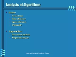
Analysis of Algorithms • Issues: • Correctness • Time efficiency • Space efficiency • Optimality • Approaches: • Theoretical analysis • Empirical analysis Design and Analysis of Algorithms - Chapter 2
input size running time Number of times basic operation is executed execution time for basic operation Theoretical analysis of time efficiency Time efficiency is analyzed by determining the number of repetitions of the basic operation as a function of input size • Basic operation: the operation that contributes most towards the running time of the algorithm. T(n) ≈copC(n) Design and Analysis of Algorithms - Chapter 2
Input size and basic operation examples Design and Analysis of Algorithms - Chapter 2
Empirical analysis of time efficiency • Select a specific (typical) sample of inputs • Use physical unit of time (e.g., milliseconds) OR • Count actual number of basic operations • Analyze the empirical data Design and Analysis of Algorithms - Chapter 2
Best-case, average-case, worst-case For some algorithms efficiency depends on type of input: • Worst case: W(n) – maximum over inputs of size n • Best case: B(n) – minimum over inputs of size n • Average case: A(n) – “average” over inputs of size n • Number of times the basic operation will be executed on typical input • NOT the average of worst and best case • Expected number of basic operations repetitions considered as a random variable under some assumption about the probability distribution of all possible inputs of size n Design and Analysis of Algorithms - Chapter 2
Example: Sequential search • Problem: Given a list of n elements and a search key K, find an element equal to K, if any. • Algorithm: Scan the list and compare its successive elements with K until either a matching element is found (successful search) of the list is exhausted (unsuccessful search) • Worst case • Best case • Average case Design and Analysis of Algorithms - Chapter 2
Types of formulas for basic operation count • Exact formula e.g., C(n) = n(n-1)/2 • Formula indicating order of growth with specific multiplicative constant e.g., C(n) ≈ 0.5 n2 • Formula indicating order of growth with unknown multiplicative constant e.g., C(n) ≈cn2 Design and Analysis of Algorithms - Chapter 2
Order of growth • Most important: Order of growth within a constant multiple as n→∞ • Example: • How much faster will algorithm run on computer that is twice as fast? • How much longer does it take to solve problem of double input size? • See table 2.1 Design and Analysis of Algorithms - Chapter 2
Table 2.1 Design and Analysis of Algorithms - Chapter 2
Asymptotic growth rate • A way of comparing functions that ignores constant factors and small input sizes • O(g(n)): class of functions f(n) that grow no faster than g(n) • Θ (g(n)): class of functions f(n) that grow at same rate as g(n) • Ω(g(n)): class of functions f(n) that grow at least as fast as g(n) see figures 2.1, 2.2, 2.3 Design and Analysis of Algorithms - Chapter 2
Big-oh Design and Analysis of Algorithms - Chapter 2
Big-omega Design and Analysis of Algorithms - Chapter 2
Big-theta Design and Analysis of Algorithms - Chapter 2
0 order of growth of T(n) ___ order of growth of g(n) c>0 order of growth of T(n) ___ order of growth of g(n) ∞ order of growth of T(n) ___ order of growth of g(n) Establishing rate of growth: Method 1 – using limits limn→∞ T(n)/g(n) = • Examples: • 10n vs. 2n2 • n(n+1)/2 vs. n2 • logb n vs. logc n Design and Analysis of Algorithms - Chapter 2
f ´(n) g ´(n) f(n) g(n) lim n→∞ lim n→∞ = L’Hôpital’s rule If • limn→∞ f(n) = limn→∞ g(n) = ∞ • The derivatives f´, g´ exist, Then • Example: logn vs. n Design and Analysis of Algorithms - Chapter 2
Establishing rate of growth: Method 2 – using definition • f(n) is O(g(n)) if order of growth of f(n) ≤ order of growth of g(n) (within constant multiple) • There exist positive constant c and non-negative integer n0 such that f(n) ≤ c g(n) for every n ≥ n0 Examples: • 10n is O(2n2) • 5n+20 is O(10n) Design and Analysis of Algorithms - Chapter 2
Basic Asymptotic Efficiency classes Design and Analysis of Algorithms - Chapter 2
Time efficiency of nonrecursive algorithms Steps in mathematical analysis of nonrecursive algorithms: • Decide on parameter n indicating input size • Identify algorithm’s basic operation • Determine worst, average, and best case for input of size n • Set up summation for C(n) reflecting algorithm’s loop structure • Simplify summation using standard formulas (see Appendix A) Design and Analysis of Algorithms - Chapter 2
Examples: • Matrix multiplication • Selection sort • Insertion sort • Mystery Algorithm Design and Analysis of Algorithms - Chapter 2
Matrix multipliacation Design and Analysis of Algorithms - Chapter 2
Selection sort Design and Analysis of Algorithms - Chapter 2
Insertion sort Design and Analysis of Algorithms - Chapter 2
Mystery algorithm for i := 1 to n - 1 do max := i ; for j := i + 1 to n do if |A[ j, i ]| > |A[ max, i ]| then max := j ; for k := i to n + 1 do swap A[ i, k ] with A[ max, k ]; for j := i + 1 to n do for k := n + 1 downto i do A[ j, k ] := A[ j, k ] - A[ i, k ] * A[ j, i ] / A[ i, i ] ; Design and Analysis of Algorithms - Chapter 2
Example Recursive evaluation of n ! • Definition: n ! = 1*2*…*(n-1)*n • Recursive definition of n!: • Algorithm: if n=0 then F(n) := 1 else F(n) := F(n-1) * n return F(n) • Recurrence for number of multiplications to compute n!: Design and Analysis of Algorithms - Chapter 2
Time efficiency of recursive algorithms Steps in mathematical analysis of recursive algorithms: • Decide on parameter n indicating input size • Identify algorithm’s basic operation • Determine worst, average, and best case for input of size n • Set up a recurrence relation and initial condition(s) for C(n)-the number of times the basic operation will be executed for an input of size n (alternatively count recursive calls). • Solve the recurrence to obtain a closed form or estimate the order of magnitude of the solution (see Appendix B) Design and Analysis of Algorithms - Chapter 2
Important recurrence types: • One (constant) operation reduces problem size by one. T(n) = T(n-1) + c T(1) = d Solution: T(n) = (n-1)c + d linear • A pass through input reduces problem size by one. T(n) = T(n-1) + cn T(1) = d Solution: T(n) = [n(n+1)/2 – 1] c + d quadratic • One (constant) operation reduces problem size by half. T(n) = T(n/2) + c T(1) = d Solution: T(n) = c lg n + d logarithmic • A pass through input reduces problem size by half. T(n) = 2T(n/2) + cn T(1) = d Solution: T(n) = cn lg n + d n n log n Design and Analysis of Algorithms - Chapter 2
A general divide-and-conquer recurrence T(n) = aT(n/b) + f (n)where f (n)∈Θ(nk) • a < bk T(n) ∈Θ(nk) • a = bk T(n) ∈Θ(nk lg n ) • a > bk T(n) ∈Θ(nlog b a) Note: the same results hold with O instead of Θ. Design and Analysis of Algorithms - Chapter 2
Fibonacci numbers • The Fibonacci sequence: 0, 1, 1, 2, 3, 5, 8, 13, 21, … • Fibonacci recurrence: F(n) = F(n-1) + F(n-2) F(0) = 0 F(1) = 1 • Another example: A(n) = 3A(n-1) - 2(n-2) A(0) = 1 A(1) = 3 • 2nd order linear homogeneous recurrence relation • with constant coefficients Design and Analysis of Algorithms - Chapter 2
Solving linear homogeneous recurrence relations with constant coefficients • Easy first: 1st order LHRRCCs: C(n) = a C(n -1) C(0) = t … Solution: C(n) = t an • Extrapolate to 2nd order L(n) = aL(n-1) + bL(n-2) … A solution?: L(n) = r n • Characteristic equation (quadratic) • Solve to obtain roots r1 and r2—e.g.:A(n) = 3A(n-1) - 2(n-2) • General solution to RR: linear combination of r1nand r2n • Particular solution: use initial conditions—e.g.:A(0) = 1 A(1) = 3 Design and Analysis of Algorithms - Chapter 2
n F(n-1) F(n) 0 1 = F(n) F(n+1) 1 1 Computing Fibonacci numbers • Definition based recursive algorithm • Nonrecursive brute-force algorithm • Explicit formula algorithm • Logarithmic algorithm based on formula: • for n≥1, assuming an efficient way of computing matrix powers. Design and Analysis of Algorithms - Chapter 2