Download
1 / 9
90 likes | 255 Views
Episode 13. Interactive computability. Hard-play machines (HPMs) Easy-play machines (EPMs) Definition of interactive computability The interactive version of the Church-Turing thesis. 0. 13.1a. Our basic model of interactive computation (game-playing by a machine) is what

E N D
Episode 13 Interactive computability • Hard-play machines (HPMs) • Easy-play machines (EPMs) • Definition of interactive computability • The interactive version of the Church-Turing thesis 0
13.1a Our basic model of interactive computation (game-playing by a machine) is what we call “hard-play machines” (HPM). Remember Turing machines (TM) model from Episode 3. We turn them into HPMs by making the following changes: From TM to HPM Valuation tape Input tape 2 0 - - - - - - - Read-only Read-write Work tape 4 0 0 - 1 # 2 $ - Read-only Run tape Output tape 4 0 0 - - - - - - No direct access Control (transition function) Move Has a finite number of states, two of which, Start and Halt, are special.
13.1b The valuation tape, serving as “static input”, spells some valuation by listing its values (separated by blanks) for all variables v0, v1, v3, ... in the alphabetical order of those variables. If only finitely many values are listed, the default value for all other variables is 0. For example, this tape spells the valuation e with e(v0)=20, e(v1)=3, e(v2)=62 and v(ei)=0 for all i3. The content of valuation tape remains unchanged throughout the work of the machine. From TM to HPM Valuation tape 2 0 - 3 - 6 2 - - Read-only Read-write Work tape 4 0 0 - 1 # 2 $ - Run tape 4 0 0 - - - - - - Read-only Control (transition function) Has a finite number of states, two of which, Start and Move, are special.
13.1c The run tape, serving as “dynamic input”, spells the current position of the play at any moment by listing its moves (in two colors). For example, this run tape spells the position400,0,1. Typically the content of this tape keeps changing (“growing”): every time a player makes a move, the move (in the corresponding color) is added to the content of the run tape. Intuitively, the function of the run tape is to make the run fully visible to the machine. From TM to HPM Valuation tape 2 0 - 3 - 6 2 - - Read-only Read-write Work tape 4 0 0 - 1 # 2 $ - Run tape 400 - 0 - 1 - - Read-only Control (transition function) Has a finite number of states, two of which, Start and Move, are special.
13.2 How an HPM works • At the beginning, the machine is in its Start state, the valuation tape spells some valuation e, the work and run tapes are blank, and the three scanning heads are in their leftmost positions. • After the computation (play) starts, the machine deterministically goes from one state to another, writes on the work tape, and moves its scanning heads left or right according to its transition function, which precisely prescribes what to do in each particular case, depending on the current state and the contents of the three scanned cells (on the three tapes). • Every time the machine enters the Move state, whatever string is to the left of the work-tape scanning head, will be automatically appended (in green color) to the content of the run tape. This means that the machine has made the move . • During each computation step, any finite number 1,...,n of red strings can also be (nondeterministically) added to the content of the run tape. This means that Environment has made the moves 1,...,n. Not limiting the number of such moves accounts for the intuition that we do not impose any conditions on the possible relative speed of the environment. • The different possibilities of the above nondeterministic updates of the run tape create different branches of computation of the machine on valuation e, and correspond to all possible scenarios of how things can evolve when the machine plays, with e on its valuation tape, against a capricious and unpredictable environment. Each branch B of computation incrementally spells some (possibly infinite) run on the run tape, which we call the run spelled byB.
13.3 Computing by an HPM Let A be a game and H be an HPM. We say that Hcomputes (or solves, or wins) A iff, for every valuation e and every computation branch B of H on e, where is the run spelled by B, we have WneA = ⊤. In other words, H computes A iff, for every valuation e (if A is not a constant game), H wins e[A] no matter how the environment behaves. H ⊧A We write to mean that H wins A. Thesis 13.1. More precisely, for every (interactive) computational problem A, we have: (a) If some HPM wins A, then A has an algorithmic (effective) solution according to everyone’s reasonable intuition. (b) If A has an algorithmic solution according to anyone’s reasonable intuition, then there is an HPM that wins A. Interactive algorithm = HPM The above is a generalization of the Church-Turing thesis to interactive problems. So, it can be called the “Interactive version of the Church-Turing thesis”.
13.4 From HPM to EPM An “easy-play machine” (EPM) is defined in the same way as an HPM, with only the following modifications: • There is an additional special state in an EPM called the permission state. We call the event of entering this state granting permission. • In the EPM model, the environment can (but is not obligated to) make a (one single) move only when the machine grants permission. • The machine is considered to win (solve, compute) a game A iff, for every valuation e and every computation branch B of the machine on that valuation, where is the run spelled by B, we have: (a) As long as Environment does not offend (does not make illegal moves of e[A]) in , the machine grants permission infinitely many times in B. (b) WneA = ⊤. Intuitions: In the EPM model, the machine has full control over the speed of its adversary --- the latter has to patiently wait for explicit permissions from the machine to make moves. The only fairness condition that the machine is expected to satisfy is that, as long as the adversary plays legal, the machine has to grant permission every once in a while; how long that “while” lasts, however, is totally up to the machine.
13.5 Of the two models of interactive computation, the HPM model is the basic one, as only it directly accounts for our intuitions that we can not or should not assume any restrictions on the behavior of the environment, including its speed. The equivalence between HPMs and EPMs But a natural question to ask is “What happens if we limit the relative speed of the environment?”. The answer turns out to be as simple as “Nothing”, as long as static games (the very entities that we agree to call computational problems) are concerned. The EPM model takes the idea of limiting the speed of the environment to the extreme, yet, according to the following theorem, it yields the same class of computable problems. Theorem 13.2. For every static game A, the following conditions are equivalent: (a) There is an HPM that computes A. (b) There is an EPM that computes A. Moreover, every HPM H can be effectively converted into an EPM E such that E wins every static game that H wins. And vice versa: every EPM E can be effectively converted into an HPM H such that H wins every static game that E wins. This theorem provides additional evidence in favor of Thesis 12.1. Even though the EPM model is equivalent to the HPM model, one of the reasons why we still want have it is that describing winning strategies in terms of EPMs is much easier than in terms of HPMs.
13.6 Throughout the previous episodes we have been abundantly using the terms “algorithmic winning strategy” (or “algorithmic solution”), “computable”, etc. It is time to at last define these most basic terms formally. Main definition Definition 13.3. Let A be a computational problem (static game). An algorithmic solution, or an algorithmic winning strategy, for A is an HPM or EPM that wins A. And A is said to be computable (winnable) iff it has an algorithmic solution. We write ⊧A to mean that A is computable.