Chapter 5 Simultaneous Linear Equations

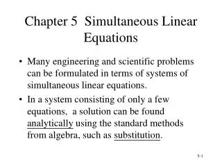
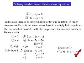
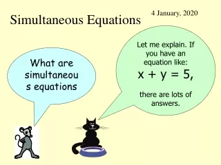
1. Chapter 5 Simultaneous Linear Equations • Many engineering and scientific problems can be formulated in terms of systems of simultaneous linear equations. • In a system consisting of only a few equations, a solution can be found analytically using the standard methods from algebra, such as substitution.

2. Example: Electrical Circuit Analysis Kirchhoff’s law I: current R: resistance V: voltage

3. Assume R1=2, R2=4, R3=5, V1=6, and V2=2. We get the following system of three linear simultaneous equations. The solution to these three equations produces the current flows in the network.

4. General Form for a System of Equations aij : known coefficient Xj : unknown variable Ci : known contant • Assume # of unknowns = # of equations • Assume the equations are linearly independent; that is, any one equation is not a linear combination of any of the other equations.

5. The linear system can be written in a matrix-vector form: Combining A and C, it can be expressed as:

6. can be expressed as:

7. Solution of Two Equations It can be solved by substitution. With substitution, we get

8. Classification of Systems of Equations • Systems that have unique solutions

9. Systems without solutions (parallel lines)

10. Systems with an infinite number of solutions (same line)

11. A system that has a solution, but has ill-conditioned parameters.

12. Permissible Operations • Rule 1: The solution is not changed if the order of the equations is changed.

13. Rule 2: Any one of the equations can be multiplied or divided by a nonzero constant without changing the solution. • Rule3: The solution is not changed if two equations are added together and the resulting equation replaces either of the two original equations.

14. Gaussian Elimination • Gaussian elimination procedure: Phase 1: forward pass Phase 2: back substitution • The the forward pass is to apply the three permissible operations to transform the original matrix to an upper-triangular matrix:

15. Written in terms of individual equations: • Back substitution:

16. Example: Gaussian Elimination Procedure Represented in the matrix form:

17. As the step 1 in the forward pass, we will convert the element a11 (a11 is called the pivot for row 1) to 1 and eliminate, that is set to zero, all the other elements in the first column.

18. Step 2: • Step 3:

19. Step 4: It represents:

20. Step 1 of backward substitution: • Step 2:

21. Step 3: • The solution is: X1 = 1, X2 = 2, X3 = 3, X4 = 4

22. Gauss-Jordan Elimination • The Gaussian elimination procedure requires a forward pass to transform the coefficient matrix into an upper-triangle form. • In Gauss-Jordan elimination, all coefficients in a column except for the pivot element are eliminated. • In Gauss-Jordan elimination, the solution is obtained directly after the forward pass; there is no back substitution phase. • The Gauss-Jordan method needs more computational effort than Gaussian elimination.

23. Example: Gauss-Jordan Elimination • Step1: • Step 2:

24. Step 3: • Step 4:

25. Accumulated Round-off Errors • Problems with round-off and truncation are most likely to occur when the coefficients in the equations differ by several orders of magnitude. • Round-off problems can be reduced by rearranging the equations such that the largest coefficient in each equation is placed on the principal diagonal of the matrix. • The equations should be ordered such that the equation having the largest pivot is reduced first, followed by the equation having the next largest, and so on.

26. Programming Gaussian Elimination • Forward pass: • Loop over each row i, making each row i in turn the pivot row. • Normalize the elements of the pivot row (row i) by dividing each element in the row by aii as follows:

27. 3.Loop over rows( i + 1) to n below the pivot row and reduce the elements in each row as follows: • Back substitution 1. For the last row n: 2. For rows (n-1) through 1,

28. LU Decomposition • A matrix A can be decomposed into L and U, where L is a lower-triangular matrix and U is a upper-triangular matrix. LU=A

29. L and U can be determined as follows:

30. AX=C LUX=C, we have LE=C and UX=E • To calculate LE=C (forward substitution) • To calculate UX=E (back substitution)

31. Relation between LU Decomposition and Gaussian Elimination • In the LU decomposition, matrix U is equivalent to the upper triangular matrix obtained in the forward pass in Gaussian elimination. • The calculation of UX=E is equivalent to the back substitution in Gaussian elimination.

32. Example: LU Decompostion Applying LU decomposition:

34. Thus, the L and U matrices are Forward substitution:

35. Back substitution:

36. Cholesky Decomposition for Symmetric Matrices • A symmetric matrix A: • Cholesky decomposition for a symmetric matrix A

37. Matrix L can be computed as follows:

38. Example: Cholesky Decomposition We can obtain the following:

40. Therefore, the L matrix is The validity can be verified as

41. Iterative Methods • Elimination methods like the Gaussian elimination procedure are often called direct equation-solving methods. An iterative method is a trial-and error procedure. • In iterative methods, we can assume a solution, that is, a set of estimates for the unknowns, and successively refine our estimate of the solution through some set of rules. • A major advantage of iterative methods is that they can be used to solve nonlinear simultaneous equations, a task that is not possible using direct elimination methods.

42. Jacobi Iteration • Each equation is rearranged to produce an expression for a single unknown.

43. Example: Jacobi Iteration Rearrange each equation as follows:

44. Assume an initial estimate for the solution: X1=X2=X3=1. First iteration: Second iteration: The solution is shown in the next table.

45. Table: Example of Jacobi Iteration

46. Gauss-Seidel Iteration • In the Jacobi iteration procedure, we always complete a full iteration cycle over all the equations before updating our solution estimates. In the Gauss-Seidel iteration procedure, we update each unknown as soon as a new estimate of that unknown is computed. • Example: Gauss-Seidel Iteration

47. Assume an initial solution estimate of X1=X2=X3=1. First iteration: Second iteration:

48. Table: Example of Gauss-Seidel Iteration Jocobi iteration method requires 13 iterations to reach the accuracy of 3 decimal places. Gauss-Seidel iteration method needs 7 iterations.

49. Convergence Considerations of the Iterative Methods • Both the Jacobi and Gauss-Seidel iterative methods may diverge. • Interchange the order of equations in the above example, and solve it by the Gauss-Seidel method:

50. Table: Divergence of Gauss-Seidel Iteration • The solution in the above table would not converge. That is, we can not get a solution. • The divergence of the iterative calculation does not imply there is no solution, since it is a permissible operation to interchange the order in a set of equations.