Download
1 / 44
440 likes | 616 Views
Solvers for Systems of Nonlinear Algebraic Equations; Where are we TODAY?. Marcin Paprzycki Oklahoma State University with Deborah Dent, Anna Kucaba-Pi ę tal and Ludomir Lauda ński. Presentation Plan. Introduction Problem description Search for the ultimate solver algorithms and solvers

E N D
Solvers for Systems of Nonlinear Algebraic Equations;Where are we TODAY? Marcin Paprzycki Oklahoma State University with Deborah Dent, Anna Kucaba-Piętal and Ludomir Laudański
Presentation Plan • Introduction • Problem description • Search for the ultimate solver • algorithms and solvers • test problems • method • small problems • large problems • Original problem revisited
Background (1) • Work originated in early 1990’s • Computer simulation of the behavior of airplanes under action of atmospheric gusts • Two possible approaches • method of harmonic (S. O. Rice) • method of filtration (N. Wiener and independently Y. A. Kchinchin) • Method of filtration used in original study
Background (2) • Result system of nonlinear algebraic equations • central/computational/difficult part of the problem • “independent” of other parts (well-defined and self-contained) • no preexisting knowledge about the solution • no simple way to suggest a starting vector • no simple way to reduce the “search area”
The Avionics Problem Filter Equation • Impulsive characteristics of a non-recursive filter h(t) as related to the correlation function K() of the stochastic process {y(t)} obtained via filtering of the input white noise {x(t)}: • K() = E [ ]
Filter Equation (2) • Since input {x(t)} is a white noise we can rewrite the problem as: • K() = for =0,1,…,N • In its explicit form we have a system of nonlinear algebraic equations
Explicit Problem Formulation K(0) = h(0)h(0) + h(1)h(1) + h(2)h(2) + … + h(N)h(N) K(1) = h(0)h(1) + h(1)h(2) + h(2)h(3) + … + h(N-1)h(N) K(2) = h(0)h(2) + h(1)h(3) + h(2)h(4) + … + h(N-2)h(N) ... K(N-2) = h(0)(N-2) + h(1)h(N-1)+h(2)h(N) K(N-1) = h(0)h(N-1) + h(1)h(N) K(N) = h(0)h(N)
Initial Work (1) • Requirements for success (engineering-estimate) • minimum N = 512 • potentially N = 1024 (?) • reached N = 64 using modified Powell’s Method (1994) • Encountered problems • computer hardware • for N = 64 solution time 10 minutes on a PC-486 • robustness of solution methods
Initial Work (2) • Research re-started questions: • how to solve the system for very (?) large N? • how to select the starting vector? • Search directions • to find (an) ultimate solver(s) • use modern hardware
Back to the Basics • System of N nonlinear algebraic equations • Large number of algorithms and implemented solvers • iterative methods • How to find the best? • use existing/agreed on test problems • compare performance • NAÏVE!
Newton’s method Powell’s algorithm Brown’s method Secant method Bisection Steepest Descent Trust Region Line Search Continuation Homotopy Augmented Lagrangian Reduced-Gradient Tensor “Available” Algorithms
Test Problems • LACK of an “all-agreed” test library ! • Test set 22 frequently used problems • some artificially generated (with properties not typical for real-life applications) • most popular More Test Set • typically small systems N 10 • only few can be extended to larger N • no problems with absolute value
Rosenbrock’s Powell singular Powell badly scaled Wood Helical Valley Watson* Chebyquad* Brown Almost-linear* Discrete Boundary Value* Discrete integral equation* Trigonometric* Variably dimensioned* Broyden tri-diagonal* Broyden banded* Exponential/Sine Function The Freudenstein-Roth Function Semiconductor Boundary Condition Brown Badly Scaled Powell singular Extended Rosenbrock Extended Matrix Square Root Problem Dennis, Gay, Vu Problem 22 Test Problems
Methodological Considerations (1) • Default settings for all solvers used • “engineering” approach • solver as black-box software • controversial choice • Test problems contain default starting vectors • additional starting vectors used • zero • one • random [0,1]
Methodological Considerations (2) • Computational cost • number of iterations • number of function evaluations • time • Two steps • problems in their default formulation • increasing the size of amenable problems
Easy test problems (solved easily by all solvers) Rosenbrock’s • Powell badly scaled Helical valley • Broyden banded function The Freudenstein-Roth Function USELESS(?!) as test problems Time so short that practically immeasurable In house codes only slightly less efficient than library solvers implementation is not the “important" issue Results (1)
Results (2) • Weakest solvers (solve only few problems outside of the easy five): • bisection • variations of Newton’s method • TENSOLVE results are slightly less accurate • Homotopy should not be used as a black-box solver • requires proper problem mapping • makes it less of a “general-purpose” solver than others
Solution of Large Problems • Test problems that can have the default number of equations increased • Watson • Chebyquad • Brown Almost-linear• Discrete Boundary Value • Discrete integral equation• Trigonometric • Variably dimensioned • Broyden tri-diagonal • Broyden banded • Five solvers left after initial selection • CONTIN • MINOS • TENSOLVE • HYBRD • LANCELOT
Results • Test problems can be divided into three groups (results for any tried starting vector): • Difficult Problems - solution only for small N ( 31) • Medium Difficult Problems - some solvers fail to reach N=1000 • Easy Problems - all solvers reach N=1000
Brown Almost Linear Discrete Boundary Value Discrete Integral Equation Trigono- metric Variably Dimen-sioned Solver Max N/ Time/Sec Max N/ Time/Sec Max N/ Time/Sec Max N/ Time/Sec Max N Time/Sec CONTIN 1000/ 300 11/ 0 4/ 0 23/ 0 4/ 0 HYBRD 22/ 0 1000/ 350 1000/ 497 40/ 0 42/ 0 TENSOLVE 1000/ 228 1000/ 1 1000/ 547 1000/ 2 200/ 31 LANCELOT 1000/ 220 1000/ 61 600/ 2826 1000/ 10506 1000/ 15 MINOS 1000/ 1094 1000/ 4 600/ 1804 1000/ 3737 1000/ 234 Medium Difficult
Sensitivity to starting vector (1) All MINOS values are > 1000
Sensitivity to starting vector (2) All MINOS values are > 1000
Observations (1) • Solvability of the problem depends on interaction between • problem • solver • starting vector • Problems not solvable using one solver with one starting vector may be solvable by another solver, or when a different starting vector is used
Observations (2) • How to detect true lack of solution to the problem? (A. Grievank, Rousse 2000) • Of the solvers tested, TENSOLVE, LANCELOT, and MINOS are most robust followed by HYBRD • CONTIN and HYBRD converge best with “default” • TENSOLVE converges best with “one” • LANCELOT and MINOS converges best with “zero”
Observations (3) • Six popular test problems: • Rosenbrock’s • Powell badly scaled • Helical valley • Broyden banded function • The Freudenstein-Roth function • Broyden tridiagonal are “easily solvable” by more robust solvers provide no useful information for performance measuring • Watson and Chebyquad seem to be very hard to solve can be recommended as real benchmarks for the robustness of new solvers • New test problems needed(?)
Original Problem Revisited • Four most robust solvers found earlier to be used: • HYBRD • TENSOLVE • LANCELOT • MINOS • Other solvers tried and similar behavior/weakness as for the test problems observed
Initial Numerical Test • Example used in original papers has solutions expressed by integers; for example • For N=2: • K(1) = 34 and K(2) = 5 • Basic solution: h(1) = 5 and h(2) = 3 • For N=4: • K(1)=30, K(2) = 20, K(3) = 11, and K(4)=4 • Basic solution: h(1)=1, h(2)=2, h(3)=3, h(4)=4 • alternate solution(!) • h(1)≈1.65, h(3≈1.58, h(3) ≈4.35, h(4) ≈2.24
Test Cases • System of equations: • K() = for j=0,1,…,N • Problem 1 Integer Data • coefficient vector created so that: • exact solution: hf (i) = i • starting vector: h0(i) = 1 • Problem 2 Floating Point Data • coefficient vector: real world data • starting vector: h0(i) = 1 • Other starting vectors used; “one” seems best-overall
HYBRD LANCELOT N IC FC Time/ sec IC FC Time/ sec 2 8 10 0 10 11 .01 4 19 27 0 8 9 .02 8 8 16 0 11 12 .04 32 10 42 0 14 15 .40 64 10 74 0 23 24 2.89 128 10 110 1 49 50 34.68 256 10 160 2 161 162 905.4 512 10 210 3 nc 1024 10 310 12 nc Results for Problem 1 (1)
MINOS TENSOLVE N IC FC Time/ sec IC FC Time/ sec 2 11 27 .01 9 23 .01 4 18 42 .01 18 42 .01 8 40 97 .01 40 94 .01 32 274 624 .32 88 201 .04 64 602 1357 2.47 274 624 2.97 128 1977 4182 19.2 602 1367 2.44 256 7340 14771 564.07 1216 2646 11.75 512 24205 47580 8346.04 4591 9422 171.02 1024 nc nc Results for Problem 1 (2)
HYBRD Converges for the largest number of equations (N = 1024) Extremely fast Best accuracy LANCELOT Converges only for up to N = 256 Slowest Different solution(!) MINOS Converges for up to N = 512 Different solution(!) TENSOLVE Converges for up to N = 512 Second fastest Solution less accurate than HYBRD Comments
HYBRD LANCELOT N IC FC Time/ sec IC FC Time/ sec 128 10 110 1 161 162 111.5 256 10 160 2 164 165 633.09 512 21 2095 90 201 206 5140.05 Results for Problem 2 (1)
MINOS TENSOLVE N IC FC Time/ sec IC FC Time/ sec 128 1068 2737 19.22 28 3818 4 256 1383 3881 131.52 16 4381 20 512 2310 6508 1068.88 12 6692 117 Results for Problem 2 (2)
Solver Minimum Error Maximum Error Average Error HYBRD 4.40E-07 7.15E-05 1.87E-05 LANCELOT 1.25E-07 5.42E-05 1.83E-05 MINOS 4.16E-07 4.45E-05 1.80E-05 TENSOLVE 4.51E-07 2.83E-03 2.86E-04 Error Estimate • Error estimate comparison between the actual coefficient vector K(i) and the computed K(i) obtained by substituting computed h(i) to the problem
509 LANCELOT 0.289799 MINOS -0.02806 TENSOLVE 0.044774790 HYBRD 0.042478349 510 0.417939 -0.03148 0.043859563 0.046436000 i x(i) x(i) x(i) x(i) 511 0.139752 -0.02624 0.027990174 0.027022607 1 -0.0596631 0.141907 -0.135745775 -0.137628574 512 0.133402 -0.06305 0.054905619 0.056642195 2 -0.0336641 0.072495 -0.080370211 -0.079030645 3 -0.0176408 0.077313 -0.074520022 -0.075754926 4 0.0450654 0.054729 -0.044292743 -0.041200875 Partial View of Solution Vectors (N= 512)
HYBRD Convergence only if TENSOLVE results used as starting vector very fast then LANCELOT Converges to a different solution MINOS Converges to yet another different solution Slowest of the three globally converging solvers TENSOLVE Converges fast Least accurate solution Accuracy improved by HYBRD as post-processor Observations
Future Work • Analysis of the three results (engineering aspects) • which/any/all solutions are “correct"? • is N = 512 enough? • what do these results mean? • Interval solver (INTLIB) for verification • Commercial solvers will they introduce anything new?
Big Picture • PROBLEM vs. SOLVER vs. STARTING VECTOR • EXISTENCE vs. NON-EXISTENCE vs. SOLUTION # • UNCONSTRAINED vs. CONSTRAINED PROBLEMS
THANK YOU! QUESTIONS?