Mining Association Rules in Large Databases
Mining Association Rules in Large Databases. What Is Association Rule Mining?. Association rule mining:

Mining Association Rules in Large Databases
E N D
Presentation Transcript
What Is Association Rule Mining? • Association rule mining: • Finding frequent patterns, associations, correlations, or causal structures among sets of items or objects in transactional databases, relational databases, and other information repositories • Motivation (market basket analysis): • If customers are buying milk, how likely is that they also buy bread? • Such rules help retailers to: • plan the shelf space: by placing milk close to bread they may increase the sales • provide advertisements/recommendation to customers that are likely to buy some products • put items that are likely to be bought together on discount, in order to increase the sales
What Is Association Rule Mining? • Applications: • Basket data analysis, cross-marketing, catalog design, loss-leader analysis, clustering, classification, etc. • Rule form: “Body ® Head [support, confidence]”. • Examples. • buys(x, “diapers”) ® buys(x, “beers”) [0.5%, 60%] • major(x, “CS”) ^ takes(x, “DB”) ® grade(x, “A”) [1%, 75%]
Association Rules: Basic Concepts • Given: (1) database of transactions, (2) each transaction is a list of items (purchased by a customer in a visit) • Find: all rules that correlate the presence of one set of items with that of another set of items • E.g., 98% of people who purchase tires and auto accessories also get automotive services done
What are the components of rules? • In data mining, a set of items is referred to as an itemset • Let D be database of transactions • e.g.: • Let I be the set of items that appear in the database, e.g., I={A,B,C,D,E,F} • A rule is defined by X Y, where XI, YI, and XY= • e.g.: {B,C} {E} is a rule
Are all the rules interesting? • The number of potential rules is huge. We may not be interested in all of them. • We are interesting in rules that: • their items appear frequently in the database • they hold with a high probability • We use the following thresholds: • the support of a rule indicates how frequently its items appear in the database • the confidence of a rule indicates the probability that if the left hand side appears in a T, also the right hand side will.
Rule Measures: Support and Confidence Customer buys both Customer buys diaper • Find all the rules X Y with minimum confidence and support • support, s, probability that a transaction contains {X Y} • confidence, c,conditional probability that a transaction having X also contains Y Customer buys beer Let minimum support 50%, and minimum confidence 50%, we have • A C (50%, 66.6%) • C A (50%, 100%)
Remember: conf(X Y) = Example • What is the support and confidence of the rule: {B,D} {A} TID date items_bought 100 10/10/99 {F,A,D,B} 200 15/10/99 {D,A,C,E,B} 300 19/10/99 {C,A,B,E} 400 20/10/99 {B,A,D} • Support: • percentage of tuples that contain {A,B,D} = 75% • Confidence: 100%
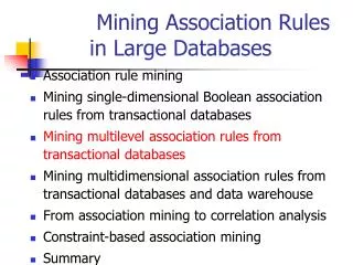
Association Rule Mining • Boolean vs. quantitative associations (Based on the types of values handled) • buys(x, “SQLServer”) ^ buys(x, “DMBook”) ® buys(x, “DBMiner”) [0.2%, 60%] • age(x, “30..39”) ^ income(x, “42..48K”) ® buys(x, “PC”) [1%, 75%] • Single dimension vs. multiple dimensional associations (see ex. Above) • Single level vs. multiple-level analysis • age(x, “30..39”) ® buys(x, “laptop”) • age(x, “30..39”) ® buys(x, “computer”) • Various extensions • Correlation, causality analysis • Association does not necessarily imply correlation or causality • Maximal frequent itemsets: no frequent supersets • frequent closed itemsets: no superset with the same support
Mining Association Rules • Two-step approach: • Frequent Itemset Generation • Generate all itemsets whose support minsup • Rule Generation • Generate high confidence rules from each frequent itemset, where each rule is a binary partitioning of a frequent itemset • Frequent itemset generation is still computationally expensive
Mining Association Rules—An Example For rule AC: support = support({AC}) = 50% confidence = support({AC})/support({A}) = 66.6% The Apriori principle: Any subset of a frequent itemset must be frequent! Min. support 50% Min. confidence 50%
Mining Frequent Itemsets: the Key Step • Find the frequent itemsets: the sets of items that have minimum support • A subset of a frequent itemset must also be a frequent itemset • i.e., if {AB} isa frequent itemset, both {A} and {B} should be a frequent itemset • Iteratively find frequent itemsets with cardinality from 1 to m (m-itemset): Use frequent k-itemsets to explore (k+1)-itemsets. • Use the frequent itemsets to generate association rules.
Level 4 (frequent quadruples): {} Level 3 (frequent triplets): {ABD}, {BDF} Level 2 (frequent pairs): {AB}, {AD}, {BF}, {BD}, {DF} {A}, {B}, {D}, {F} Level 1 (frequent items): Remember: All subsets of a frequent itemset must be frequent Visualization of the level-wise process: Question: Can ADF be frequent? NO: because AF is not frequent
The Apriori Algorithm (the general idea) • Find frequent items and put them to Lk (k=1) • Use Lk to generate a collection of candidate itemsets Ck+1 with size (k+1) • Scan the database to find which itemsets in Ck+1 are frequent and put them into Lk+1 • If Lk+1 is not empty • k=k+1 • GOTO 2
The Apriori Algorithm • Pseudo-code: Ck: Candidate itemset of size k Lk : frequent itemset of size k L1 = {frequent items}; for(k = 1; Lk !=; k++) do begin Ck+1 = candidates generated from Lk; for each transaction t in database do increment the count of all candidates in Ck+1 that are contained in t Lk+1 = candidates in Ck+1 with min_support (frequent) end returnkLk; • Important steps in candidate generation: • Join Step: Ck+1is generated by joining Lk with itself • Prune Step: Any k-itemset that is not frequent cannot be a subset of a frequent (k+1)-itemset
The Apriori Algorithm — Example Database D L1 C1 Scan D min_sup=2=50% C2 C2 L2 Scan D L3 C3 Scan D
How to Generate Candidates? • Suppose the items in Lk are listed in an order • Step 1: self-joining Lk(IN SQL) insert intoCk+1 select p.item1, p.item2, …, p.itemk, q.itemk from Lk p, Lk q where p.item1=q.item1, …, p.itemk-1=q.itemk-1, p.itemk < q.itemk • Step 2: pruning forall itemsets c in Ck+1do forall k-subsets s of c do if (s is not in Lk) then delete c from Ck+1
{a,c,d} {a,c,e} {a,c,d,e} cde acd ace ade X Example of Candidates Generation • L3={abc, abd, acd, ace, bcd} • Self-joining: L3*L3 • abcd from abc and abd • acde from acd and ace • Pruning: • acde is removed because ade is not in L3 • C4={abcd} X
How to Count Supports of Candidates? • Why counting supports of candidates a problem? • The total number of candidates can be huge • One transaction may contain many candidates • Method: • Candidate itemsets are stored in a hash-tree • Leaf nodeof hash-tree contains a list of itemsets and counts • Interior node contains a hash table • Subset function: finds all the candidates contained in a transaction
H H H H H Example of the hash-tree for C3 Hash function: mod 3 Hash on 1st item 2,5,.. 3,6,.. 1,4,.. 234 567 Hash on 2nd item 145 356 689 345 367 368 Hash on 3rd item 124 457 125 458 159
H H H H H Example of the hash-tree for C3 2345 look for 2XX 345 look for 3XX Hash function: mod 3 12345 Hash on 1st item 12345 look for 1XX 2,5,.. 3,6,.. 1,4,.. 234 567 Hash on 2nd item 145 356 689 345 367 368 Hash on 3rd item 124 457 125 458 159
H H H H H Example of the hash-tree for C3 2345 look for 2XX 345 look for 3XX Hash function: mod 3 12345 Hash on 1st item 12345 look for 1XX 2,5,.. 3,6,.. 1,4,.. 234 567 Hash on 2nd item 12345 look for 12X 145 356 689 345 367 368 12345 look for 13X (null) 124 457 125 458 159 12345 look for 14X
AprioriTid: Use D only for first pass • The database is not used after the 1st pass. • Instead, the set Ck’ is used for each step, Ck’ = <TID, {Xk}> : each Xk is a potentially frequent itemset in transaction with id=TID. • At each step Ck’ is generated from Ck-1’ at the pruning step of constructing Ck and used to compute Lk. • For small values of k, Ck’ could be larger than the database!
AprioriTid Example (min_sup=2) L1 C1’ Database D C1’ L2 C2 L3 C3 C3’
Methods to Improve Apriori’s Efficiency • Hash-based itemset counting: A k-itemset whose corresponding hashing bucket count is below the threshold cannot be frequent • Transaction reduction: A transaction that does not contain any frequent k-itemset is useless in subsequent scans • Partitioning: Any itemset that is potentially frequent in DB must be frequent in at least one of the partitions of DB • Sampling: mining on a subset of given data, lower support threshold + a method to determine the completeness • Dynamic itemset counting: add new candidate itemsets only when all of their subsets are estimated to be frequent
Illustrating Apriori Principle Found to be Infrequent Pruned supersets
Factors Affecting Complexity • Choice of minimum support threshold • lowering support threshold results in more frequent itemsets • this may increase number of candidates and max length of frequent itemsets • Dimensionality (number of items) of the data set • more space is needed to store support count of each item • if number of frequent items also increases, both computation and I/O costs may also increase • Size of database • since Apriori makes multiple passes, run time of algorithm may increase with number of transactions • Average transaction width • transaction width increases with denser data sets • This may increase max length of frequent itemsets and traversals of hash tree (number of subsets in a transaction increases with its width)
Rule Generation • Given a frequent itemset L, find all non-empty subsets f L such that f L – f satisfies the minimum confidence requirement • If {A,B,C,D} is a frequent itemset, candidate rules: ABC D, ABD C, ACD B, BCD A, A BCD, B ACD, C ABD, D ABCAB CD, AC BD, AD BC, BC AD, BD AC, CD AB, • If |L| = k, then there are 2k – 2 candidate association rules (ignoring L and L)
Rule Generation • How to efficiently generate rules from frequent itemsets? • In general, confidence does not have an anti-monotone property c(ABC D) can be larger or smaller than c(AB D) • But confidence of rules generated from the same itemset has an anti-monotone property • e.g., L = {A,B,C,D}: c(ABC D) c(AB CD) c(A BCD) • Confidence is anti-monotone w.r.t. number of items on the RHS of the rule
Pruned Rules Rule Generation for Apriori Algorithm Lattice of rules Low Confidence Rule
Rule Generation for Apriori Algorithm • Candidate rule is generated by merging two rules that share the same prefixin the rule consequent • join(CD=>AB,BD=>AC)would produce the candidaterule D => ABC • Prune rule D=>ABC if itssubset AD=>BC does not havehigh confidence