Download
1 / 34
340 likes | 355 Views
This course provides an overview of digital speech processing, including topics such as linguistic processing and latent topic analysis. The course is taught by Professor Lin-Shan Lee from National Taiwan University.

E N D
數位語音處理概論 Introduction to Digital Speech Processing 14.0 Linguistic Processing and Latent Topic Analysis 【本著作除另有註明外,採取創用CC「姓名標示-非商業性-相同方式分享」臺灣3.0版授權釋出】 授課教師:國立臺灣大學 電機工程學系 李琳山 教授
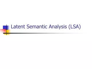
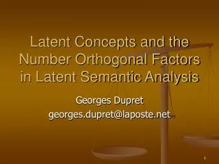
Latent Semantic Analysis (LSA) Tk Topic Documents Words
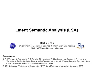
d1 d2 ........dj.......... dN w1 w2 . wi wM wij Latent Semantic Analysis (LSA) - Word-Document Matrix Representation • Vocabulary V of size M and Corpus T of size N • V={w1,w2,...wi,..wM} , wi: the i-th word ,e.g. M=2×10⁴ T={d1,d2,...dj,..dN} , dj: the j-th document ,e.g. N=105 • cij: number of times wi occurs in dj nj: total number of words present in dj ti= Σjcij : total number of times wi occurs in T • Word-Document Matrix W W = [wij] • each row of W is a N-dim “feature vector” for a word wiwith respect to all documents dj each column of W is a M-dim “feature vector” for a document djwith respect to all words wi 3
T 2 Dimensionality Reduction (1/2) • dimensionality reduction: selection of R largest eigenvalues (R=800 for example) R “concepts” or “latent semantic concepts” 5
Dimensionality Reduction (2/2) T 2 T • dimensionality reduction: selection of R largest eigenvalues (i, j) element of WT W : inner product of i-th and j-th columns of W “similarity” between di and dj T N N si2: weights (significance of the “component matrices” e′ie′iT) R “concepts” or “latent semantic concepts” 6
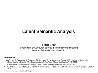
d1 d2 ........ dj. ......... dN d1 d2 ........ dj.......... dN w1 w2 wi wM s1 T vj VT sR U = wij R×R R×N ui M×R w1 w2 wi wM Singular Value Decomposition (SVD) • Singular Value Decomposition (SVD) • si: singular values, s1≥ s2.... ≥ sR U: left singular matrix, V: right singular matrix • Vectors for word wi: uiS=ui (a row) • a vector with dimensionality N reduced to a vector uiS=ui with dimensionality R • N-dimensional space defined by N documents reduced to R-dimensional space defined by R “concepts” • the R row vectors of VT, or column vectors of V, or eigenvectors {e′1,..e′R}, are the R orthonormal basis for the “latent semantic space” with dimensionality R, with which uiS = uiis represented • words with similar “semantic concepts” have “closer” location in the “latent semantic space” • they tend to appear in similar “types” of documents, although not necessarily in exactly the same documents 7
Singular Value Decomposition (SVD) • dp=USvpT (just as a column in W= USVT) 8
d1 d2 ........ dj . ......... dN d1 d2 ........ dj.......... dN w1 w2 wi wM s1 T vj VT U sR wij R×R = R×N ui M×R w1 w2 wi wM Singular Value Decomposition (SVD) • Singular Value Decomposition (SVD) • Vectors for document dj: vjS=vj(a row, or vj= S vjTfor a column) • a vector with dimentionality M reduced to a vector vjS=vjwith dimentionality R • M-dimentional space defined by M words reduced to R-dimentional space defined by R “concepts” • the R columns of U, or eigenvectors{e1,...eR}, are the R orthonormal basis for the “latent semantic space” with dimensionality R, with which vjS=vjis represented • documents with similar “semantic concepts” have “closer” location in the “latent semantic space” • they tend to include similar “types” of words, although not necessarily exactly the same words • The Association Structure between words wiand documentsdj is preserved with noisy information deleted, while the dimensionality is reduced to a common set of R “concepts” T 9
Example Applications in Linguistic Processing • Word Clustering • example applications: class-based language modeling, information retrieval ,etc. • words with similar “semantic concepts” have “closer” location in the “latent semantic space” • they tend to appear in similar “types” of documents, although not necessarily in exactly the same documents • each component in the reduced word vector ujS=ujis the “association” of the word with the corresponding “concept” • example similarity measure between two words: • Document Clustering • example applications: clustered language modeling, language model adaptation, information retrieval, etc. • documents with similar “semantic concepts” have “closer” location in the “latent semantic space” • they tend to include similar “types” of words, although not necessarily exactly the same words • each component on the reduced document vector vjS=vjis the “association” of the document with the corresponding “concept” • example “similarity” measure between two documents: 2 2 10
LSA for Linguistic Processing Cosine Similarity if magnitude Similarity 11
Example Applications in Linguistic Processing • Information Retrieval • “concept matching” vs “lexical matching” : relevant documents are associated with similar “concepts”, but may not include exactly the same words • example approach: treating the query as a new document (by “folding-in”), and evaluating its “similarity” with all possible documents • Fold-in • consider a new document outside of the training corpus T, but with similar language patterns or “concepts” • construct a new column dp ,p>N, with respect to the M words • assuming U and S remain unchanged dp=USvpT (just as a column in W= USVT) vp = vpS= dpTU as an R-dim representation of the new document (i.e. obtaining the projection of dp on the basis ei of U by inner product) 12
T i-th dimensionality out of M Integration with N-gram Language Models • Language Modeling for Speech Recognition • Prob(wq|dq-1) wq: the q-th word in the current document to be recognized (q: sequence index) dq-1: the recognized history in the current document vq-1=dq-1TU : representation of dq-1 by vq-1 (folded-in) • Prob(wq|dq-1) can be estimated by uqandvq-1 in the R-dim space • integration with N-gram Prob(wq|Hq-1) =Prob(wq|hq-1,dq-1) Hq-1: history up to wq-1 hq-1:<wq-n+1, wq-n+2,... wq-1 > • N-gram gives local relationships, while dq-1 gives semantic concepts • dq-1 emphasizes more the key content words, while N-gram counts all words similarly including function words • vq-1 for dq-1 can be estimated iteratively • assuming the q-th word in the current document is wi (n) (n) vq moves in the R-dim space initially, eventually settle down somewhere 13
Probabilistic Latent Semantic Analysis (PLSA) Di:documents Tk: latent topics tj: terms • Exactly the same as LSA, using a set of latent topics{ }to construct a new relationship between the documents and terms, but with a probabilistic framework • Trained with EM by maximizing the total likelihood • : frequency count of term in the document 14
Probabilistic Latent Semantic Analysis (PLSA) w: word z: topic d: document N: words in document d M: documents in corpus 15
Latent Dirichlet Allocation(LDA) : Dirichlet Distribution : prior for ) : Dirichlet Distribution : prior for ( k: topic index, a total of K topics ) • A document is represented as random mixtures of latent topics • Each topic is characterized by a distribution over words 16
Gibbs Sampling in general • To obtain a distribution of a given form with unknown parameters • Initialize • For • Sample ~ Take a sample of base on the distribution • Sample ~ • Sample ~ • Sample ~ • Apply MarKov Chain Monte Carlo and sample each variable sequentially conditioned on the other variables until the distribution converges, then estimate the parameters based on the coverged distribution 17
Gibbs Sampling applied on LDA • Sample P(Z,W) : ? ? ? ? Topic … w11 w12 w13 w1n ? ? ? ? Word Doc 1 … w21 w22 w23 w2n Doc 2 … 18
Gibbs Sampling applied on LDA • Sample P(Z,W) : • Random Initialization … w11 w12 w13 w1n Doc 1 … w21 w22 w23 w2n Doc 2 … 19
Gibbs Sampling applied on LDA ? … w11 w12 w13 w1n • Sample P(Z,W) : • Random Initialization • Erase Z11, and draw a new Z11 ~ Doc 1 … w21 w22 w23 w2n Doc 2 … 20
Gibbs Sampling applied on LDA ? … w11 w12 w13 w1n • Sample P(Z,W) : • Random Initialization • Erase Z11, and draw a new Z11 ~ • Erase Z12, and draw a new Z12 ~ Doc 1 … w21 w22 w23 w2n Doc 2 … 21
Gibbs Sampling applied on LDA • Sample P(Z,W) : • Random Initialization • Erase Z11, and draw a new Z11 ~ • Erase Z12, and draw a new Z12 ~ … w11 w12 w13 w1n Doc 1 … w21 w22 w23 w2n Doc 2 … • Iteratively update topic assignment for each word until converge • Compute θ, φ according to the final setting 22
Matrix Factorization (MF) for Recommendation systems : rating u:user i:item 23
Matrix Factorization (MF) • Mapping both users and items to a joint latent factor space of dimensionality f f I I 1 1 i i 1 1 f latent factor: towards male, seriousness, etc. = u u U U 24
Matrix Factorization (MF) • Objective function • Training • gradient decent (GD) • Alternating least square (ALS): alternatively fix ’s or ’s and compute the other as a least square problem • Different from SVD (LSA) • SVD assumes missing entries to be zero (a poor assumption) 25
Overfitting Problem • A good model is not just to fit all the training data • needs to cover unseen data well which may have distributions slightly different from that of training data • too complicated models with too many parameters usually leads to overfitting 26
Extensions of Matrix Factorization (MF) • Biased MF • add global bias μ(usually = average rating), user biasbu, and item bias bias parameters • Non-negative Matrix Factorization • restrict the value in each component of pu and qito be non-negative 27
References • LSA and PLSA • “Exploiting Latent Semantic Information in Statistical Language Modeling”, Proceedings of the IEEE, Aug 2000 • “Latent Semantic Mapping”, IEEE Signal Processing Magazine, Sept. 2005, Special Issue on Speech Technology in Human-Machine Communication • “Probabilistic Latent Semantic Indexing”, ACM Special Interest Group on Information Retrieval (ACM SIGIR), 1999 • “Probabilistic Latent Semantic Indexing”, Proc. of Uncertainty in Artificial Intelligence, 1999 • “Spoken Document Understanding and Organization”, IEEE Signal Processing Magazine, Sept. 2005, Special Issue on Speech Technology in Human-Machine Communication • LDA and Gibbs Sampling • Christopher M. Bishop, Pattern Recognition and Machine Learning, Springer 2006 • Blei, David M.; Andrew Y. Ng, Michael I. Jordan. "Latent Dirichlet Allocation”, Journal of Machine Learning Research 2003 • Gregor Heinrich, ”Parameter estimation for text analysis”, 2005 28
References • Matrix Factorization • A Linear Ensemble of Individual and Blended Models for Music Rating Prediction. In JMLR W&CP, volume 18, 2011. • Y. Koren, R. M. Bell, and C. Volinsky. Matrix factorization techniques for recommender systems. Computer, 42(8):30-37, 2009. • Introduction to Matrix Factorization Methods Collaborative Filtering (http://www.intelligentmining.com/knowledge/slides/Collaborative.Filtering.Factorization.pdf) • GraphLab API: Collaborative Filtering (http://docs.graphlab.org/collaborative_filtering.html) • J Mairal, F Bach, J Ponce, G Sapiro, Online learning for matrix factorization and sparse coding, The Journal of Machine Learning, 2010 29
版權聲明 30
版權聲明 31
版權聲明 32
版權聲明 33
版權聲明 34