Download
1 / 57
570 likes | 678 Views
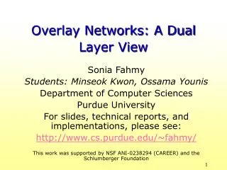
Overlay Networks: A Dual Layer View. Sonia Fahmy Students: Minseok Kwon, Ossama Younis Department of Computer Sciences Purdue University For slides, technical reports, and implementations, please see: http://www.cs.purdue.edu/~fahmy/

E N D
Overlay Networks: A Dual Layer View Sonia Fahmy Students: Minseok Kwon, Ossama Younis Department of Computer Sciences Purdue University For slides, technical reports, and implementations, please see: http://www.cs.purdue.edu/~fahmy/ This work was supported by NSF ANI-0238294 (CAREER) and the Schlumberger Foundation
Why Overlays? • Overlay networks help overcome deployment barriers to network-level solutions • The advantages of overlays include flexibility, adaptivity, and ease of deployment • Applications • Application-level multicast (e.g., End System Multicast/Narada) • Inter-domain routing pathology solutions (e.g., Resilient Overlay Networks) • Content distribution • Peer-to-peer networks
Overlay Multicast Overlay link Receivers Source Routers and underlying links
Characterizing Overlay Networks Why Characterize Overlays? • Overlay multicast consumes additional network bandwidth and increases latency over IP multicast quantify the overlay performance penalty • Little work has been done on characterizing overlay multicast tree structure, especially large trees • Such characterization gives insight into overlay properties and their causes, and a deeper understanding of different overlay multicast approaches better overlay design Real data from ESM experiments Analytical models Simulations
Our Hypothesis • Observations • Many high degree high bandwidth routers heavily utilized in upper levels of ESM/TAG trees, which tend to be longer. Many hosts are connected to lower degree low bandwidth routers, clustered close together at lower levels of the trees. This lowers multicast cost • Causes • Overlay host distribution • Overlay protocol (full/partial info/overhead, delay/bandwidth/diameter/degree, source-based/shared tree/trees/mesh) • Topology (connectivity and degrees)
Overlay Tree Metrics • Overlay cost = number of underlying hops traversed by every overlay link • Link stress = total number of identical copies of a packet over the same underlying link • Overlay cost = ∑stress(i) for all router-to-router links i • Number of hops and delays between parent and child hosts in an overlay tree • Degree of hosts = host contribution to the link stress of the host-to-first-router link • Degree of routers and hop-by-hop delays of underlying links traversed by overlay links • Mean bottleneck bandwidth between the source and receivers • Relative Delay Penalty (RDP), mean/longest latency
Overlay link Receivers Source C 20 ms B A 10 ms • Overlay cost = 12 • Link stress on A = 2 • RDP of B = (15+15+10)/20 = 2 15 ms 15 ms Metrics: Examples
Overlay Tree Structure • Questions • What do overlay multicast trees look like? Why? • How much additional cost do they incur over IP multicast? • Methodology • Use overlay trees (65 hosts) in ESM experiments (from CMU) in November 2002. Use public traceroute servers and synthesize approximate routes. (Most university hosts are connected to the Internet 2 backbone network) • PlanetLab experiments and tree/traceroute data
Results: End System Multicast • Distributions of per-hop delay for different overlay tree levels • Number of hops between two hosts versus level of host in overlay trees (a) Tree level 1 (b) Tree levels 4-6
Results: End System Multicast • Frequency of occurrence of number of hop values between two hosts • Degree of host versus level of host in overlay tree
Experiments on PlanetLab • Internet Experiments • Implement and experiment with TAG (Topology-Aware Grouping) on the PlanetLab (http://www.planet-lab.org) wide-area platform • Additional experiments with NICE and HyperCast • Run several sets of experiments with nodes in the United States, Europe, and Asia
Overlay Tree Structure: Simulations • Topologies • Contains 4k routers connected in ways consistent with router-level power-law and small-world properties • GT-ITM topology with 4k routers • Delays and bandwidths according to realistic distributions • Overlay multicast algorithms • ESM (End System Multicast) [SIGCOMM 2001] • A host has the upper degree bound (we use 6) on the number of its neighbors • TAG (Topology-Aware Grouping) [extended NOSSDAV 2002] • Uses ulimit=6 and bwthresh=100 kbps for partial path matching • MDDBST (Minimum Diameter Degree-Bounded Spanning Tree) [NOSSDAV 2001, INFOCOM 2003] • Minimizes the number of hops in the longest path, and bounds the degree of hosts in overlay trees (degree bound = edge bw/min bw)
Results: Number of Hops • Non-uniform host distribution • Uniform host distribution MDDBST not as clear as ESM, because it minimizes max. cost
Results: Isolation of Topology Effects • Variability in router degrees • Clustering (small world)
Results: Degree • Router degree versus overlay tree level of destination host • Frequency of router degree
Results: Latency and Bandwidth • Relative delay penalty (RDP) • Mean bottleneck bandwidth ESM achieves a good balance, but scalability is a concern
Overlay Multicast Tree Cost Source • Network Model • LO(h,k,n) denotes overlay cost for an overlay O when n is the number of hosts • We only count hops in router subsequences • We use n instead of m • Why an underlying tree model? • Simple analysis • Consistency with real topologies [Radoslavov00] • Transformation from a graph to a k-ary tree with minimum cost tree • Why least cost tree? • Modeling and analysis are simplified • Many overlay multicast algorithms optimize a delay-related metric, which is typically also optimized by underlying intra-domain routing protocols • A lower bound on the overlay tree cost can be computed k h Host Receiver
Network Models with Unary Nodes Branching node Unary node with only one child Number of unary nodes created between adjacent nodes at levels i-1 and i Self-similar Tree Model(k=2, θ=1, h=3) • To incorporate the number-of-hops distribution, use a self-similar tree model [SODA2002]
Level l α k (b) Receivers at Leaf Nodes Source k r Overlay link h α Receiver (a)
Receivers at Leaf Nodes The overlay cost in (a): The overlay cost in (b): where where if otherwise The sum of (a) and (b): n1-θis observed
Receivers at Leaf Nodes where θ=0.15
α k(1-p) kp (A) … … β Level l kp … (B) … (b) Receivers at Leaf or Non-leaf Nodes kp k(1-p) … … kp α k(1-p) … … β h k(1-p) kp Lυ(h-1,k,n) L υ(h-2,k,n) L υ(h-3,k,n) (a)
Receivers at Leaf or Non-leaf Nodes The overlay cost in (a): The overlay cost in (b): where The sum of (a) and (b):
Receivers at Leaf or Non-leaf Nodes where θ=0.15
Cost Model Validation • The analytical results are validated using traceroute-based simulation topologies and our earlier topologies • Normalized overly cost via simulations • ESM and MDDBST have n0.8-n0.9; TAG has a slightly higher cost due to partial path matching • Cost with GT-ITM/uniform hosts is higher than with non-uniform/power-law/small-world • The normalized overlay tree cost for the real ESM tree is n0.945
Related Work • Chuang and Sirbu (1998) found that the ratio between the total number of multicast links and the average unicast path length exhibits a power-law (m0.8) • Chalmers and Almeroth (2001) found the ratio to be around m0.7and multicast trees have a high frequency of unary nodes • Phillips et al.(1999), Adjih et al.(2002) and Mieghem et al.(2001) mathematically model the efficiency of IP multicast • Radoslavov (2000) characterized real and generated topologies with respect to neighborhood size growth, robustness, and increase in path lengths due to link failure. They analyzed the impact of topology on heuristic overlay multicast strategies • Jin and Bestavros (2002) have shown that both Internet AS-level and router-level graphs exhibit small-world behavior. They also outlined how small-world behavior affects the overlay multicast tree size • Overlay multicast algorithms include End System Multicast (2000,2001), CAN-based multicast (2002), MDDBST (2001,2003), TAG (2001), etc.
Conclusions • We have investigated the efficiency of overlay multicast using theoretical models, experimental data, and simulations. We find that: • The number of routers/delay between parent and child hosts tends to decrease as the level of the host in the ESM/TAG overlay tree increaseslower cost • Routing features in overlay multicast protocols, non-uniform host distribution, along with power-law and small-world topology characteristics contribute to these phenomena • We can quantify potential bandwidth savings of overlay multicast compared to unicast (n0.9 < n) and the bandwidth penalty of overlay multicast compared to IP multicast (n0.9 > n0.8)
Ongoing Work • We are conducting larger scale simulations and experiments using PlanetLab • We are examining other and more dynamic metrics with other overlay protocols • We will precisely formulate the relationship between the overlay trees, overlay protocols and Internet topology characteristics • We are investigating the possibility of inter-overlay cooperation to further reduce the overlay performance penalty
Other Work… • Exploiting network tomography for monitoring and traffic engineering • FlowMate on-line passive flow clustering: design and implementation [ICNP 2002, ToN] • Distributed network delay and loss monitoring [CC 2003] • Testing security mechanisms [Computers&Security 2003, CACM 2004] • Sensor networks [INFOCOM 2004, IWQoS 2004]
Cooperative Overlays Overlay A Overlays A and B may or may not cooperate. Co-located nodes Overlay B Shared routers and links
A Spectrum of Overlay Cooperation Less cooperation More cooperation Independent overlays Merged overlays Sharing information e.g., control info, queries Shared measurement Cooperative forwarding Inter-overlay Traffic engineering
Route X Route Y Cooperative Forwarding Overlay A Overlay B • Route Y is better than route X which only uses hosts in overlay A. Can be proactive or reactive for long-lived flows.
Cooperation Mechanisms • Privilege levels • Full privileges and obligations: a host (active member) is authorized to use all the services provided by its home overlay network(s). • Limited privileges and obligations: a host (passive member) has limited capabilities such as routing and replication. • Each overlay selects a set of nodes that other overlays can exploit as passive members (transit nodes) according to peering relationships. • Inter-overlay agents selected according to: • Number of co-located overlay nodes; Number of different overlays represented in neighbor nodes; Minimum maximum delay to other hosts in home overlay • Passive membership selected according to: • Performance improvement of other overlays, e.g., Number of members that have this passive member as their next hop (maximum-next-hop) • Compatibility and loads of other overlays • Trust-based priority to determine which overlays are cooperative
Additional Cooperative Services • Shared measurement service • Control information sharing (e.g., randomized routing time intervals and traffic equilibrium computation for multiple overlays) • Query forwarding in peer-to-peer networks • Inter-overlay traffic engineering
Related Work • Overlay broadcasting (Y. Chawathe et al.) • Studies possibility of cooperation among overlays. • Routing underlay (A. Nakao et al.) • Provides shared network layer information to overlay nodes. • Tomography-based overlay network monitoring (Y. Chen et al.) • Requires O(n) measurements for all the O(n2) overlay paths. • Selfish source and overlay routing (L. Qiu et al.) • Other overlay networks • Include RON, Detour, End System Multicast, etc.
Current Plan • We are designing a cooperative overlay architecture for heterogeneous overlay networks to collaborate. • Our goal is to prove that overlay cooperation reduces competition, improves overall performance, and preserves heterogeneity [ICNP2003 poster]. • Ongoing Work • We are currently implementing our algorithms on PlanetLab. • We will examine other types of overlay cooperation services with particular attention to the complexity, scalability, and security issues.
Is “On-line” Tomography Useful and at What Time Scale? What is “tomography”? A method of producing (inferring) an image of the internalstructures of a solid object by the observation and recording of the differences in the effects on the passage of waves of energy impinging on those structures. What is “network tomography”? Internet mapping (routes, per-segment delays, per-segment losses, per-segment bandwidth, shared bottlenecks) via composing end-to-end measurements.
Why FlowMate? Receiver Receiver Source Receiver Receiver
Why FlowMate? • Partitioning flows emerging from the same source (busy server) according to shared bottlenecks is useful for: • Customized, more fair and more responsive coordinated congestion management. • Overlay networks (e.g., application-layer multicast and peer-to-peer applications). • Load balancing. • Pricing. • Traffic engineering and admission control.
The Problem • Input: • A set of flows (micro or macro), F, originating at the same source, where F = {f1, f2, …, fn} • Required: • Periodically map each flow fi (1 i n) to a cluster gj (1 j m) G = {g1, g2, …, gm}, mn, where all flows fgj G share a common bottleneck
FlowMate Features • Employs passive probing to reduce probe generation and processing overhead, and network load with a large number of flows. • Employs on-line clustering based on constantly changing shared bottlenecks. • Works with or without receiver timestamp support (and no router support). • Reduces overhead using representatives. • Uses limited history for stability (no samples).
Architecture Transport layer implementation enables more accurate timestamping
Basic Algorithm [O(NG)] Initialize: Empty cluster list and flow table. Repeat forever: - Collect delay Information. - Check triggering condition. - If (triggered): cluster flows and generate clusters. - Delete delay samples and maintain compact history information. Partitioning: - Select delay samples. - Assign a representative flow for each cluster. - Each flow is tested against each representative, and joins the cluster with highest correlation. - A flow either joins a cluster or forms a new one.
Shared Bottleneck Test For two flows f1 and f2 sharing a common bottleneck in sr [Rubenstein00]:The cross correlation measure of multiplexed (f1, f2) packets, spaced apart by time t > 0, is higher than the auto correlation measure of packets of f1 or f2, spaced apart by time T > t. r s
In-Band Delay Sampling • One way delay (reasonable clock skew OK). • Extend the time-stamped ACK (RFC 1323) to include packet reception time. • Select samples according to inter-packet spacing. Samples chosen as probes time
Last time clustering was invoked Clustering may be invoked if enough samples for all flows Time t d_min d_max Clustering must be invoked if not invoked since t Clustering not invoked Triggering Clustering • Every flow with at least M samples is considered
Our Accuracy Index • Sources of inaccuracies: false sharing and cluster splits • A cluster split is not as harmful as false sharing Let kj denote the resulting number of splits of a correct cluster: Example: correct: {1,2,3},{4,5,6}, result: {1,2},{3,4,5},{6}, I=0.67
D1 4 ms bottlenecks 2 22 ms D2 3 ms Cross- traffic generator 1 D3 1.5 Mbps 3 4 5 ms 3 ms 11 ms D4 17 ms 12 ms 1 ms Source 19 ms 5 ms 9 ms 13 ms s 5 6 7 8 2 ms 2 ms 3 Mbps 3 ms 3 ms D5 D8 D7 D6 10 Mbps 14 ms D9 5 ms 10 12 ms D10 3 ms 9 D11 4 ms 14 ms 12 ms 11 D12 2 ms Cross- traffic destination(s) Simulation Configuration Configuration: • Cross and reverse traffic: CBR sources • Forward traffic: FTP, Telnet, or HTTP/1.1 • Background traffic: 3 “StarWars” flows (self-similar traffic)
Foreground Load FlowMate accuracy (using a simpler topology) Different loads Staggered start times Correlation periods: 1, 2, 4, 6, 8, 10 seconds.
Background Load • Load and on/off periods have little impact on average accuracy