Monitoring and program evaluation

1. Monitoring and program evaluation Hossein Naraghi CE 590 Special Topics Safety June 2003 Time spent:9 hrs

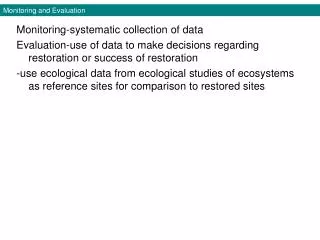
2. The need fro monitoring • Monitoring is systematic collection of data about the performance of road safety treatments after their implementation • The effectiveness of treatment can be assessed • Post-implementation monitoring is essential to ascertain the effects of a treatment • Improve the accuracy and confidence of predictions of that treatment’s effectiveness in subsequent applications

3. The need fro monitoring (continued) • Monitoring is important to ensure that a particular treatment has not led to a significant increase in accidents • The road safety engineer has a duty to ensure that the public does not experiencing additional hazard as a result of treatments • The Institution of Highways and Transportation defines the purpose of monitoring as follow • Assess the effects of crash occurrence in relation to safety objectives

4. The need fro monitoring (continued) • Assess the effects on distribution of traffic and speeds of motor vehicle • Call attention to any unintended effects on traffic movement or accident occurrence • Assess the effect of treatment on the local environment • Find out about the public response to the treatment in terms of its acceptability in general and people’s concern about safety in particular

5. The need fro monitoring (continued) • The County Surveyors’ Society 1991 suggests three ways for monitoring a site • Pay careful attention to a site immediately after treatment • In case things go badly wrong • Assess the effect over a longer time period • About three years to determine the influence of treatment on crashes or other performance measures • This needs careful statistical analysis to correct for external factors

6. The need fro monitoring (continued) • Focus on the accident types which the treatment was intended to correct • Assess whether these have in fact declined • Monitoring and evaluation is meaningful if • there has been a clear statement of objectives of the treatment • A prediction of its effects • A logical link between treatment and its effects • Monitoring should apply to all accident investigation and prevention work

7. The need fro monitoring (continued) • Road safety treatments potentially affect the following parameters which need to be monitored • The number and type of crashes • The severity of crashes • The distribution of crashes over the road network • Traffic flows and travel times • Turning movements and delays at intersections • Access times and distances within residential areas • Route taken by motorists, cyclists and pedestrians • Operation of buses

8. The need fro monitoring (continued) • A comprehensive monitoring practice should involve all these effects • Since crashes are relatively rare event, it may take a very long time to acquire a statistically reliable sample, which makes monitoring difficult • This can be partially overcome by the use of proxy measures such as • Traffic conflict measures • Indirect measures • Insurance company claim record • Emergency service records • Ambulance, hospital admission • Tow truck records

9. The need fro monitoring (continued) • Resources devoted to monitoring in most agencies are limited • Resources should be devoted directly to development and implementation of treatments which have been prioritized and shown to have potential for crash reduction rather than monitoring exercises • We should admit that our understanding of safety effectiveness of road safety engineering treatments is limited and in many cases rests on shaky foundation

10. The need fro monitoring (continued) • This point comprehensively argued by Hauer 1988, who says that • “the level of safety built into roads is largely unpremeditated. Standards and practices have evolved without a foundation of knowledge. At times the safety consequences of engineering decisions are not known, at others some knowledge exists but not used.”

11. Monitoring techniques • The essence of monitoring is to measure what is happening in the real world. There are several experimental challenges in doing this • There may be changes in road environment • Change in speed limit • Change in traffic flow • Change in abutting land uses • Change in traffic control • Since crashes are rare and randomly occurring events, there will be year by year fluctuations which have nothing to do with the treatment being analyzed

12. Monitoring techniques (continued) • It is necessary to monitor all significant factors which might affect the outcome • If two variables are systematically related and both are measured, it will not be possible to reliably isolate their independent effects • Statistical correlation does not necessary imply logical correlation • Ensure a linkage between the treatment being monitored and the change in performance measure • Seasonal factors must be taken into account

13. Monitoring techniques (continued) • It would be incorrect to compare the summer (before) accident record with the winter (after) accident record if one was trying to assess the effect of skid-resistance • Accident reporting levels may change over time, and there may be inconsistencies in accident data which need to be considered • There may be a long term trend in crash occurrence, therefore changes over time in the rate of crashes at a site may merely reflect global trends • It is usually necessary to use some form of control group and compare crashes at the site with those at the control site

14. Monitoring techniques (continued) • There are four ways that the evaluation of the effect of a road safety treatment can be done • Controlled experimentation • All other factors held constant except the factor whose effect is being investigated • This approach is rarely applicable in road safety engineering, because in the real world it is not possible to hold everything constant • Before and after studies • Comparisons using control sites • Time trend comparisons

15. Before and after studies • Is the simplest and least satisfactory method because of the lack of control of extraneous factors and essentially involves • Determining in advance the relevant objectives (e.g. accident types intended to be affected) and the corresponding evaluation criteria (e.g. accident frequency, accident rate) • Monitoring the site to obtain numerical values for these criteria before and after treatment • Comparing the before and after results • Considering whether there are other plausible explanations for the change and correct them

16. Before and after studies (continued) • Any before and after study, usually relies on pre-existing data • This underlies the need for systematic on-going data collection, so the effect of changes can be monitored routinely • Statistical analysis of data should be carefully undertaken with regard to accuracy of data • It will be helpful to consider more than just changes in accident frequency of the particular accident type • It may also be useful to check the changes in the 85 percentile values, variance, skew, etc

17. Before and after studies (continued) • For any formal before and after study to be statistically valid, a reasonable period of time must be considered to obtain a sufficient sample • While one year may be considered a minimum analysis period, three years is generally regarded as a reasonable period for trends to be established and a sufficiently large sample obtained • Nicholson (1987) recommended 5 years for statistical confidence

18. Comparisons using control sites • The problem of before and after study is that it takes no account for changes across the network as a whole • This can be overcome by using the control sites • There are two variations using control sites • Using control group which are randomly selected • A controlled experiment by selecting several candidate sites foe a particular treatment in advance

19. Comparisons using control sites (continued) • Then they are randomly split into two groups • All sites in the first group and no sites in the second group are treated • The objective here is to make control and treatment groups equal in all factors except for the execution of treatment • Two groups do not need to be of equal size, but they must satisfy sample size requirements • This method is powerful as an investigation tool • It is of limited validity for most applications in roads safety engineering • There will barely be the opportunity to conduct a controlled experiment of this nature

20. Comparisons using control sites (continued) • Using selected comparison groups • Involves a before and after study • The result of before and after study will be compared with the result of the control site • The process involves: • Specifying the objectives in advance • Identifying a set of control sites • No remedial work have been or intended to be introduced • Monitoring both the treated and control sites before and after treatment to obtain numerical values

21. Comparisons using control sites (continued) • Comparing the before and after results at both the treated and control sites • Considering if there other plausible explanations for the changes and correct them if possible • Selection of control sites is very important in this process and should satisfy the following criteria: • Be similar to treated sites in general characteristics • Network configuration • Geometric standards • Land use

22. Comparisons using control sites (continued) • Socio-economic characteristics • Enforcement practices, etc • Be geographically close • Have similar traffic flows • Not affected by treatment at the test site • Not be treated in any way in the period of before and after study • Have crash record which are consistent in both collection criteria and coding covering the period of study • A useful device is simply graph the number of crash after against the number crash before treatment at both test & control sites (Figure 17.1 page 444)

23. Time trend comparison • This method involves the development of a model to estimate the trend of accident over time which involves the following process: • Identifying the objectives in advance and the corresponding analysis criteria • Obtaining data on each criteria for an extended period of time • Developing a model based on the before period • Comparing projections based upon the model for after period with the measured criteria for that period • Identifying if there are other plausible explanations for the changes and correct them

24. Time trend comparison (continued) • This method is useful where substantial countermeasure has been produced at a given point in time • Limited application in road safety engineering, since it is very difficult to control for all variables in real world analysis • Analytical power of this approach has been much extended by the development of log-linear models

25. Analysis of accident statistics • Three main applications of statistical testing in the area of road safety engineering are as follow: • Comparison of crash frequencies • A chi-squared test is suitable • Or a paired t-test if the distribution of crashes can be assumed to be normal • Comparison of crash rates • A paired t-test is appropriate • Comparison of proportions • A z-test is suitable (See table 17.1 page 447)

26. Analysis of accident statistics (continued) • Poisson distribution is a very simple test for calculating probabilities • Can be used in determining whether a specific crash frequency is within the bounds of normal year by year fluctuations • Methodological issues • There are four important methodological issues • Regression to the mean • Accident migration • Risk compensation • Sample size determination

27. Regression to mean • Over a period of time, if there are no changes in physical or traffic characteristics at a site, annual crashes at that site tend to fluctuate about the mean value due to the random nature of crash occurrence • Since the selected sites for treatment are based on their ranking in number of crashes compare to all other sites, there is a high possibility that sites will be chosen when their crash count is higher than long term average • The crash rates at these sites is likely to experience a lower rate in the following year even without implementing any treatment

28. Regression to mean (continued) • This aspect of crash experience need to be concerned in after implementation analysis of a safety treatment • Since this phenomenon is present, the impact of treatment will be exaggerated • Regression to mean may exaggerate the effect of a treatment from 5-30 percent • Since our knowledge of safety effects of treatment built up from the results of this kind of studies, therefore there is a tendency to over-state the effectiveness of road and traffic engineering treatment

29. Regression to mean (continued) • This sometimes called “bias by selection” (Hauer 1980) • Analysts are responsible to separate the real benefits from a particular treatment from the changes due to regression to mean phenomenon • The problem can be substantially minimized by increasing the number of years of data used in the site selection process • This does not solve the problem entirely • It is not always expedient to wait for several years before conducting an evaluation exercise

30. Regression to mean (continued) • To correct for regression to mean phenomenon, the true underlying accident rate should be estimated • There are two common approaches • Model the accident situation in order to estimate the true underlying accident rate and then based the evaluation on the model not the raw accident data • Multi-variate modeling approach developed by Hauer (1983, 1992) • Adjust the data to correct for biases using assumptions about the statistical distribution of accidents year by year

31. Regression to mean (continued) • Multi-variate modeling approach which extends the Empirical Bayes model to allow “unsafety” to be estimated when a large reference population does not exist • The model can be described as follows: • If XB and XA are respectively the accident frequencies observed before and after treatment at a site which prior to treatment had an underlying mean accident frequency m, then the treatment effect, t is given by: t = XA / m And the regression to the mean effect, r by: r = m / XB

32. Regression to mean (continued) • If regression to the mean effects are ignored it is assumed that m = XB however, rather than using data for study site itself to estimate m, the Empirical Bayes approach uses the following expression m = a + bxB

33. Accident migration • The assumption here is that accidents may increase at sites surrounding the treated site due to changes in trip pattern or driver’s assessment of risk • A study in a sample of sites in London show that accident at the treated sites fell by 22%, but accident in the surrounding street increased by 10% • The effect of remedial measure for this phenomenon is to relocate the accidents not to reduce them • A statistical explanation for this phenomenon showing that there is a spatial correlation between accident frequencies at adjacent or nearby sites, so use of neighboring sites as control sites leads to bias

34. Risk compensation • Road users adjust their behavior as they perceive the road system • One factor that affect the behavior is perception of risk • If the the road is perceived as more hazardous then drivers may respond accordingly • Reducing speed in icy condition • Some of the additional road safety provided as a result of road safety treatment is used up by drivers behaving in a more risky manner • To make sense of the risk notion in the context of road safety engineering, it is important to distinguish between objective and subjective risks

35. Risk compensation (continued) • Objective risk • Perceived risk • Subjective risk • What affects behavior • A road safety treatment may • Reduce the objective risk and increase the subjective risk • e.g. set of traffic signals both alerts drivers to the hazard presented by the intersection and moderating the hazard by separating conflicting streams of traffic • Increase subjective risk alone • e.g. warning sign effectiveness depends entirely on driver response

36. Risk compensation (continued) • Reduce the objective risk alone • e.g. skid resistance pavements are not usually discernible to the driver • Reduce both objective risk and subjective risk • e.g. improved road geometry, improved sight distance, grade separation, etc • It is only in this category that risk compensation could be a factor, in other categories there is either no change in subjective risk or an increase in it • Any road design change which reduces the subjective risk should also reduce the objective risk to at least the same extent, otherwise the road user will have a tendency to respond inappropriately

37. Sample size determination • The smaller the change in accident at any site, the larger is the sample necessary to determine the statistical significance • In evaluating a countermeasure, the analyst must use either a longer time period or a larger number of sites • The sample size required depends on • The effect that analyst seek to detect • e.g. whether the treatment is expected to decrease accidents by 10%, 20%, 50% or so on • The probability of detecting a real effect • The level of significance

38. Sample size determination (continued) • All feasible combinations of these three factors will produce a multitude of outcomes (see table 17.2 page 463)