Overpotential
230 likes | 982 Views
Overpotential. When the cell is balanced against an external source, the Galvani potential difference, ∆ Φ , can be identified as the electrode zero-current potential, E. When the cell is producing current, the electrode potential changes from its zero-current value, E, to a new value, E’.

Overpotential
E N D
Presentation Transcript
Overpotential • When the cell is balanced against an external source, the Galvani potential difference, ∆Φ , can be identified as the electrode zero-current potential, E. • When the cell is producing current, the electrode potential changes from its zero-current value, E, to a new value, E’. • The difference between E and E’ is the electrode’s overpotential, η. η = E’ – E • The ∆Φ = η + E, • Expressing current density in terms of η ja = j0e(1-a)fη and jc = j0e-afη where jo is called the exchange current density, which is when there is no net current flow, i.e. ja = jc
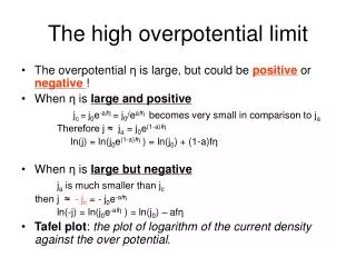
The Butler-Volmer equation: j = j0(e(1-a)fη - e-afη) • The low overpotential limit η < 0.01 V • The high overpotential limit η ≥ 0.12 V
The low overpotential limit • The overpotential ηis very small, i.e. fη <<1 • When x is small, ex = 1 + x + … • Therefore ja = j0[1 + (1-a) fη] jc = j0[1 + (-a fη)] • Then j = ja - jc = j0[1 + (1-a) fη] - j0[1 + (-a fη)] = j0fη • The above equation illustrates that at low overpotential limit, the current density is proportional to the overpotential. • It is important to know how the overpotential determines the property of the current.
Calculations under low overpotential conditions • Example 25.2: The exchange current density of a Pt(s)|H2(g)|H+(aq) electrode at 298K is 0.79 mAcm-2. Calculate the current density when the over potential is +5.0mV. Solution: j0 = 0.79 mAcm-2 η = 5.0mV f = F/RT = j = j0fη • Self-test 25.6: What would be the current at pH = 2.0, the other conditions being the same?
The high overpotential limit • The overpotential ηis large, but could be positive or negative ! • When η is large and positive jc =j0e-afη= j0/eafη becomes very small in comparison to ja Therefore j ≈ ja = j0e(1-a)fη ln(j) = ln(j0e(1-a)fη ) = ln(j0) + (1-a)fη • When η is large but negative ja is much smaller than jc then j ≈ - jc = - j0e-afη ln(-j) = ln(j0e-afη ) = ln(j0) – afη • Tafel plot: the plot of logarithm of the current density against the over potential.
Applications of a Tafel plot • The following data are the anodic current through a platinum electrode of area 2.0 cm2 in contact with an Fe3+, Fe2+ aqueous solution at 298K. Calculate the exchange current density and the transfer coefficient for the process. η/mV 50 100 150 200 250 I/mA 8.8 25 58 131 298 Solution: calculate j0 and α Note that I needs to be converted to J
Self-test 25.7: Repeat the analysis using the following cathodic current data: η/mV -50 -100 -150 -200 -250 I/mA -0.3 -1.5 -6.4 -27.61 -118.6 • In general exchange currents are large when the redox process involves no bond breaking or if only weak bonds are broken. • Exchange currents are generally small when more than one electron needs to be transferred, or multiple or strong bonds are broken.
The general arrangement for electrochemical rate measurement
25.10 Voltammetry • Voltammetry: the current is monitored as the potential of the electrode is changed. • Chronopotentiometry: the potential is monitored as the current density is changed. • Voltammetry may also be used to identify species and determine their concentration in solution. • Non-polarizable electrode: their potential only slightly changes when a current passes through them. Such as calomel and H2/Pt electrodes • Polarizable electrodes: those with strongly current-dependent potentials. • A criterion for low polarizability is high exchange current density due to j = j0fη
Concentration polarization • At low current density, the conversion of the electroactive species is negligible. • At high current density the consumption of electroactive species close to the electrode results in a concentration gradient. • Concentration polarization: The consumption of electroactive species close to the electrode results in a concentration gradient and diffusion of the species towards the electrode from the bulk may become rate-determining. Therefore, a large overpotential is needed to produce a given current. • Polarization overpotential: ηc
Consider the reduction half reaction: Mz+ + ze → M • The Nernst equation is E = Eө + (RT/zF) ln(a) • When using a large excess of support electrolyte, the mean activity coefficients stays approximately constant, E = Eө + (RT/zF)ln(γ) + (RT/zF)ln(c) E = Eo + (RT/zF)ln(c) • The ion concentration at OHP decreases to c’ due to the reaction, resulting E’ = Eo + (RT/zF)ln(c’) • The concentration overpotential is ηc = E’ – E = (RT/zF)ln(c’/c) (typo in the 8th edition)
The thickness of the Nernst diffusion layer (illustrated in previous slide) is typically 0.1 mm, and depends strongly on the condition of hydrodynamic flow due to such as stirring or convective effects. • The Nernst diffusion layer is different from the electric double layer, which is typically less than 1 nm. • The concentration gradient through the Nernst diffusion layer is dc/dx = (c’ – c)/δ • This concentration gradient gives rise to a flux of ions towards the electrode J = - D(dc/dx) • Therefore, the particle flux toward the electrode is J = D (c – c’)/ δ
The cathodic current density towards the electrode is the product of the particle flux and the charge transferred per mole of ions (zF) j = zFJ = zFD(c – c’)/ δ • The maximum rate of diffusion across the Nernst layer is when c’ = 0 at which the concentration gradient is the steepest. jlim = zFJ = zFDc/ δ • Using the Nerst-Einstein equation (D = RTλ/(zF)2), jlim = cRTλ/(zFδ) where λ is ionic conductivity
Example 25.3: Estimate the limiting current density at 298K for an electrode in a 0.10M Cu2+(aq) unstirred solution in which the thickness of the diffusion layer is about 0.3mm. • Solution: one needs to know the following information molar conductivity of Cu2+: λ = 107 S cm2 mol-1 δ = 0.3 mm employing the following equation: jlim = cRTλ/(zFδ) • Self-test 25.8 Evaluate the limiting current density for an Ag(s)/Ag+(aq) electrode in 0.010 mol dm-3 Ag+(aq) at 298K. Take δ = 0.03mm.
From j = zFD(c – c’)/ δ, one gets c’ = c - jδ/zFD • ηc = (RT/zF)ln(c’/c) = (RT/zF)ln(1 - jδ/(zFDc)) • Or j = (zFDc)(1 – ezfη)/δ