Coding Programs by Numbers

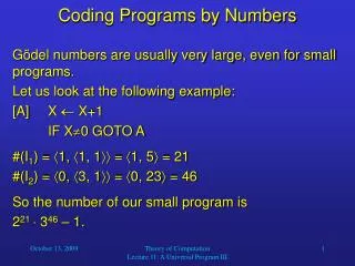
1. Coding Programs by Numbers Gödel numbers are usually very large, even for small programs. Let us look at the following example: [A] X  X+1 IF X0 GOTO A #(I1) = 1, 1, 1 = 1, 5 = 21 #(I2) = 0, 3, 1 = 0, 23 = 46 So the number of our small program is 221  346 – 1. Theory of Computation Lecture 11: A Universal Program III

2. Coding Programs by Numbers Note that the number of the unlabeled instruction Y  Y is 0, 0, 0 = 0, 0 = 0. Thus, the number of a program will be unchanged if an unlabeled instruction Y  Y is appended to it. Although this ambiguity is harmless, we avoid it by adding a sentence to our definition of programs of L : The final instruction in a program is not permitted to be the unlabeled statement Y  Y. Theory of Computation Lecture 11: A Universal Program III

3. Coding Programs by Numbers Then each number determines a unique program. As an example, let us determine the program whose number is 199: 199 + 1 = 200 = 23  30  52 = [3, 0, 2]. So if #(P ) = 199, P consists of 3 instructions, the second of which is the unlabeled statement Y  Y. 3 = 2, 0 = 2, 0, 0 2 = 0, 1 = 0, 1, 0 Thus, the program is: [B] Y  Y Y  Y Y  Y+1 Theory of Computation Lecture 11: A Universal Program III

4. The Halting Problem Let us define the predicate HALT(x, y). For a given number y, let P be the program such that #(P ) = y. Then HALT(x, y) is true if P(1)(x) is defined and false if P(1)(x) is undefined. In other words: HALT(x, y)  program number y eventually halts on input x. Here comes a surprise: Theorem 2.1: HALT(x, y) is not a computable predicate. Theory of Computation Lecture 11: A Universal Program III

5. The Halting Problem Proof (by contradiction): Assume that HALT(x, y) were computable. Then we could write the following program P : [A] IF HALT(X, X) GOTO A This program P would compute the following function: P(1)(x) =  if HALT(x, x) = 0 if HALT(x, x) Now let #(P ) = y0. Then by the definition of HALT we get: HALT(x, y0)  HALT(x, x) For input x = y0 we then have: HALT(y0, y0)  HALT(y0, y0) Contradiction! Theory of Computation Lecture 11: A Universal Program III

6. The Halting Problem So finally we have an example of a predicate that is not computable by any program in the language L . We would even like to conclude the following: There is no algorithm that, given a program of L and an input to that program, can determine whether or not the given program will eventually halt on the given input. This is called the unsolvability of the halting problem. Theory of Computation Lecture 11: A Universal Program III

7. The Halting Problem • If there were such an algorithm, we could use it to determine the truth value of HALT(x, y) for given x and y: • We would first obtain the program Q so that #(Q ) = y. • Then we would check whether Q eventually halts on input x. • However, we have reason to believe that any algorithm for computing on numbers can be carried out by a program of L (Church’s Thesis). • So this would contradict the fact that HALT(x, y) is not computable. Theory of Computation Lecture 11: A Universal Program III

8. The Halting Problem It may surprise you that there is no algorithm for solving the halting problem. Is it not possible for a computer scientist to analyze a given program and find out whether it will terminate for a particular input or not (even if this analysis takes a very long time)? No, actually we can devise a very simple program in L for which to date nobody is able to tell whether it will ever terminate. Theory of Computation Lecture 11: A Universal Program III

9. The Halting Problem This program is based on Goldbach’s conjecture, which assumes that every even number  4 is the sum of two prime numbers. For example, 4 = 2 + 2, 6 = 3 + 3, 48 = 41 + 7. It would be easy to write a program in L that searches for a counterexample to this conjecture. This program would check the following predicate for increasing values n: (x)n(y)n[Prime(x) & Prime(y) & x + y = n] Nobody knows whether this program will ever halt. Theory of Computation Lecture 11: A Universal Program III

10. Universality For each n > 0, let us define: (n)(x1, …, xn, y) = P(n)(x1, …, xn) , where #(P ) = y. Theorem 3.1 (Universality Theorem): For each n > 0, the function (n)(x1, …, xn, y) is partially computable. This is one of the most important theorems in computability theory. We will prove it by providing instructions for writing a program Un that computes (n) for each n > 0. Theory of Computation Lecture 11: A Universal Program III

11. Universality In other words, for each n > 0 we want to have: Un(n+1)(x1, …, xn, xn+1) = (n)(x1, …, xn, xn+1) . These programs Un are called universal. For example, U1 can be used to compute any partially computable function of one variable. If there is a program P that computes f(x), and #(P ) = y, then f(x) = (1)(x, y) = U1(2)(x, y). It is useful to think of the programs Un in terms of interpreters of programs in L . Theory of Computation Lecture 11: A Universal Program III

12. Universality • The universal programs must • decode the number of the program given to them, • keep track of the current snapshot during program execution, and • generate the next snapshot based on the current one and the current instruction. • When we write such programs, we will freely use macros referring to functions that we already know to be primitive recursive. • We will also freely use label and variable names beyond those specified for the language L . Theory of Computation Lecture 11: A Universal Program III

13. Universality In describing the state of a computation, we assume all variables to have the value 0 if not assigned a different value. Then we can code the state of the computation by the Gödel number [a1, …, am], where ai is the value of the i-th variable in our ordered list. Obviously, m is chosen so that all ai for i > m are 0. For example, the state Y = 1, X = 2, Z2 = 1 is coded by the following number: [1, 2, 0, 0, 1] = 2  32  11 = 198. Theory of Computation Lecture 11: A Universal Program III

14. Universality • In order to store the current snapshot, we need to keep track of two numbers: • K is the number of the instruction to be executed next, and • S is the current state coded as a Gödel number (see previous slide). • Now we are ready to write the program Un for computing Y = (n)(X1, …, Xn, Xn+1). • We will explain Un piece by piece and finally put the pieces together. Theory of Computation Lecture 11: A Universal Program III

15. Universality Z  Xn+1 + 1 S  ni=1 (p2i)Xi K  1 If Xn+1 = #(P ), where P consists of the instructions I1, …, Im, then Z = [#(I1), …, #(Im)]. S is initialized as [0, X1, 0, X2, …, 0, Xn], which puts the input values into the first n input variables and 0s into the other variables. K is given the value 1 so that the computation will begin with the first instruction. Theory of Computation Lecture 11: A Universal Program III

16. Universality Then we append the following instruction: [C] IF K = Lt(Z) + 1  K = 0 GOTO F So if the computation has ended, GOTO F, where the proper value will be output. Otherwise, the current instruction is decoded and executed: U  r((Z)K) P  pr(U)+1 Remember that (Z)K = a, b, c is the number of the K-th instruction. So U = b, c is the code of the statement to be executed. The variable mentioned in this statement is the (c + 1)-th, i.e., the (r(U) + 1)-th. Theory of Computation Lecture 11: A Universal Program III