Download
1 / 64
640 likes | 796 Views
This document delves into advanced scheduling policies for real-time operating systems, focusing on Rate Monotonic Scheduling (RMS) and Earliest Deadline First (EDF) methodologies. It outlines modeling assumptions, key performance metrics like CPU utilization and scheduling overhead, and challenges like priority inversion and interprocess communication. The document covers how to evaluate scheduling policies, implement them efficiently, and deal with issues arising from unschedulable processes. A technical overview of POSIX scheduling is included, alongside practical examples and solutions to common scheduling problems.

E N D
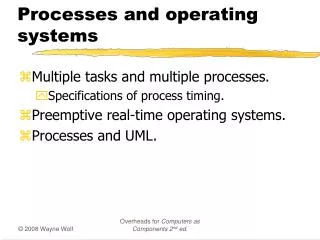
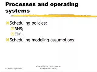
Processes and operating systems • Scheduling policies: RMS EDF- Scheduling modeling assumptions.- Interprocess communication.- Power management.
Metrics • How do we evaluate a scheduling policy: • Ability to satisfy all deadlines. • CPU utilization---percentage of time devoted to useful work. • Scheduling overhead---time required to make scheduling decision. • themore sophisticated the scheduling policy, the more CPU time it takes during system operation.
POSIX #include <sched.h> int i, my_process_id; Struct sched_param my_sched_params; … … i = sched_setscheduler(my_process_id, SCHED_FIFO, &sched_params);
Rate monotonic scheduling • RMS (Liu and Layland): widely-used, analyzable scheduling policy. • Analysis is known as Rate Monotonic Analysis (RMA).
RMA model • Assumptions • All process run on single CPU. • Zero context switch time. • No data dependencies between processes. • Process execution time is constant. • Deadline is at end of period. • Highest-priority ready process runs.
Ci Ci Ci i period Ti Process parameters • Ci is computation time of process ti; Ti is period of process ti.
Rate-monotonic analysis • Response time: time required to finish process. • Critical instant: scheduling state that gives worst response time. • Critical instant occurs when all higher-priority processes are ready to execute.
interfering processes P1 P1 P1 P1 P2 P2 P3 Critical instant P1 P2 P3 critical instant P4
RMS priorities • Optimal (fixed) priority assignment: • shortest-period process gets highest priority; • priority inversely proportional to period; • break ties arbitrarily. • No fixed-priority scheme does better.
1 C1 C1 C1 4 8 2 C2 C2 time 0 5 10 RMS example
RMS CPU utilization • Utilization for n processes is • S = (1, 2, …, n) • U = Si=1..n Ci / Ti
Utilization 1.0 0.828 0.78 0.69 nTasks Rate Monotonic, Liu & Layland, 1973 • For a configuration of n periodic tasks to be scheduled, a sufficient condition for schedulability is: All n tasks are schedulable if U ≤ n ( 21/n - 1) As number of tasks approaches infinity, maximum utilization approaches 69%.
예외적인 경우의 예 C1 C1 C1 C1 C1 1 (C1/T1=1/2) 2 4 6 8 C2 C2 2 (C2/T2=1/4) 0 4 8 C3 C3 3 (C3/T3=2/8) 0 8 time U = ½ + ¼ + 1/8 = 1 3(21/3 -1) = 0.78
RMS CPU utilization, cont’d. • RMS cannot asymptotically guarantee 100% use of CPU, even with zero context switch overhead. • Must keep idle cycles available to handle worst-case scenario. • However, RMS guarantees all processes will always meet their deadlines.
RMS implementation • Efficient implementation: • scan processes; • choose highest-priority active process.
Earliest-deadline-first scheduling • EDF: dynamic priority scheduling scheme. • Process closest to its deadline has highest priority. • Requires recalculating process priority at every timer interrupt.
EDF example 1 2
EDF analysis • EDF can use 100% of CPU. • If U <= 1, a given set of tasks is schedulable • But EDF may miss a deadline due to some scheduling overhead.
EDF implementation • On each timer interrupt: • compute time to deadline; • choose process closest to deadline. • Generally considered too expensive to use in practice.
Fixing scheduling problems • What if your set of processes is unschedulable? • Change deadlines in requirements. • Reduce execution times of processes. • Get a faster CPU.
Priority inversion • Priority inversion: low-priority process keeps high-priority process from running. • Improper use of system resources can cause scheduling problems: • Low-priority process grabs I/O device. • High-priority device needs I/O device, but can’t get it until low-priority process is done. • Can cause deadlock.
Task priority Priority Inversion: Example • Comment: • The interruption of task 2 which is generated by task 1 is normal since task 1 has a higher priority than task 2. • The interruption generated by task 2 is an incorrect behavior of the scheduler.
Solving priority inversion • Give priorities to system resources. • Have process inherit the priority of a resource that it requests. • Low-priority process inherits priority of device if higher.
Priority Inheritance Protocol • The resource management protocol is: •if the resource is free: a task gets the resource •if the resource is not free: the task is blocked and the task needing the resource inherits the priority of the blocked task Task 2
Task priority w/o using Priority Inheritance Protocol
with using Priority Inheritance Protocol • Management of the tasks by priority inheritance to avoid the expected need for a critical resource: the task 0 was delayed by the task 2 with lower priority. • The temporal sequence is modified by the fact that task 3 takes the priority equals of task 0 (inherit) when this one needs the resource already allocated to task 3. This inheritance of the priority allows task3 to release the critical resource as early as possible and thus task 0 to finish its execution without execution of the task 2.
Priority Inheritance Protocol: example • Task 2 is at most delayed by the longest critical section of task 3 • Bi inf(n, m).CRmax
Data dependencies allow us to improve utilization. Restrict combination of processes that can run simultaneously. P1 and P2 can’t run simultaneously. Data dependencies 1 2 P1 P3 P2 What if P3 has higher priority than P1 and P2? P3 can interfere with only one of these twos.
Context-switching time • Non-zero context switch time can push limits of a tight schedule. • Hard to calculate effects---depends on order of context switches. • In practice, OS context switch overhead is small.
What about interrupts? • Interrupts take time away from processes. • Perform minimum work possible in the interrupt handler. P1 OS P2 intr OS P3
Device processing structure • Interrupt service routine (ISR) performs minimal I/O. • Get register values, put register values. • Interrupt service process/thread performs most of device function.
POSIX scheduling policies • SCHED_FIFO: RMS • SCHED_RR: round-robin • within a priority level, processes are time-sliced in round-robin fashion • The length of quantum can vary with priority level • SCHED_OTHER: undefined scheduling policy used to mix non-real-time and real-time processes.
Interprocess communication • OS provides interprocess communication mechanisms: • various efficiencies; • communication power. • Types • Shared memory • Message passing • Signal (Unix)
Signals • A Unix mechanism for simple communication between processes. • Analogous to an interrupt---forces execution of a process at a given location. • But a signal is caused by one process with a function call • No data---can only pass type of signal.
POSIX signal types • Termination • SIGABRT: abort • SIGTERM: terminate process • Exceptions • SIGFPE: floating point exception • SIGILL: illegal instruction • SIGKILL: unavoidable process termination • User-defined • SIGUSR1, SIGUSR2: user defined • Etc…
POSIX signals • Must declare a signal handler for the process using sigaction(). • Handler is called when signal is received. • A signal can be sent with sigqueue().
Non-real-time signal program in Posix #include <signal.h> extern void usr1_handler(int); // declare SIGUSR1 handler struct sigaction act, oldact; int retval; //setup the descriptor data structure act.sa_flags = 0; sigemptyset(&act.sa_mask); // initilize the signal set to empty act.sa_handler = usr1_handler; // add SIGUSR1 handler to the set //tell the OS about this handler retval = sigaction(SIGUSR1, &act, &oldact); // oldact has old action set
Real-time Signals (POSIX.4) • Range [SIGRTMIN, SIGRTMAX] • If (sigqueue(destpid, SIGRTMAX - 1, sval) < 0) { • //error • } • ** Queuing can be turned on using the SA_SIGINFO bit in the sa_flags field of the sigaction structure.
Signals in UML • More general than Unix signal---may carry arbitrary data: someClass <<signal>> aSig <<send>> sigbehavior() p : integer aSig object indicated by the <<signal>> streotype
POSIX Semaphore • POSIX supports counting semaphores with _POSIX_SEMAPHORES option. • Semaphore with N resources will not block until N processes hold the semaphore. • Semaphores are given name: • /sem1 • P() is sem_wait(), V() is sem_post().
POSIC Semaphore • int i, oflags; • sem_t *my_sem; • my_sem = sem_open(“/sem1”, oflags); //create a new one • //Do useful works • i = sem_close(my_sem); //remove the semaphore • int i; • i = sem_wait(my_sem); • //access critial section • i= sem_post(my_sem); • //test w/o blocking • i=sem_trywait(my_sem);
POSIX Shared Memory // only one process open these two function calls objdesc = shm_open(“/memobj1”, O_RDWR); //cf. O_RDONLY if (ftrucate(objdesc, 1000) < 0) { //set the size of the shared memory //error } // all processes that wants to use the shared memory have use the mmap if (mmap(addr, len, O_RDWR, MAP_SHARED, objdesc, 0) == NULL) { //error } If (munmap(startadrs, len) < 0 {//error} close (objdesc); // dispose of the shared memory All processes call mmap(), munmap(). Only one process calls shm_open(), close().
POSIC mmap() function parameters len startaddr len objdesc offset objdesc Backing store Memory
POSIX message-based communication • Unix pipe supports messages between processes. • Parent process uses pipe() to create a pipe. • Pipe is created before child is created so that pipe ID can be passed to child.
POSIX pipe example /* create the pipe */ if (pipe(pipe_ends) < 0) //return an array of file descriptors, pipe_ends[0] and pipe_ends[1] { perror(“pipe”); break; } //pipe_ends[0] for the write end, pipe_ends[1] for the rea end /* create the process */ childid = fork(); if (childid == 0) { /* child reads from pipe_ends[1] */ //pass the read ebd descriptor to the new incarnation of child childargs[0] = pipe_ends[1]; //file descriptor execv(“mychild”,childargs); perror(“execv”); exit(1); } else { /* parent writes to pipe_ends[0] */ … } * Parent writes something using pipe_ends[0] and child reads it using pipe_ends[1].
Cache Effects (cache mgmt) Each process use half the cache. Use LRU policy. How many cache-miss? P1 P1 P2 P2 P3 P3 In cache: P1 P1, P2 P2, P3 P1, P3 P2, P1 P3, P2 What if we reserve half the cache for P1?
Evaluating performance • May want to test: • context switch time assumptions; • scheduling policy. • Can use OS simulator to exercise a set of process, trace system behavior.
Processes and caches • Processes can cause additional caching problems. • Even if individual processes are well-behaved, processes may interfere with each other. • Execution time with bad cache behavior is usually much worse than execution time with good cache behavior.
Power optimization • Power management: determining how system resources are scheduled/used to control power consumption. • OS can manage for power just as it manages for time. • OS reduces power by shutting down units. • May have partial shutdown modes.
Power management and performance • Power management and performance are often at odds • Entering power-down mode consumes • energy, • time. • Leaving power-down mode consumes • energy, • time.