Parametric Equations
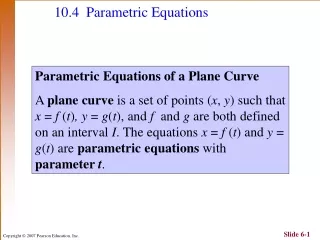
Parametric Equations. Lesson 6.7. Movement of an Object. Consider the position of an object as a function of time The x coordinate is a function of time x = f(t) The y coordinate is a function of time y = g(t). •. •. time. 0. Table of Values. We have t as an independent variable

Parametric Equations
E N D
Presentation Transcript
Parametric Equations Lesson 6.7
Movement of an Object • Consider the position of an object as a function of time • The x coordinate is a function of timex = f(t) • The y coordinate is a function of timey = g(t) • • time 0
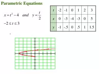
Table of Values • We have t as an independent variable • Both x and y are dependent variables • Given • x = 3t • y = t2 + 4 • Complete the table
Plotting the Points • Use the Data Matrix on the TI calculator • Choose APPS, 6, and Current • Data matrix appears • Use F1, 8 to clear previous values
Plotting the Points • Enter the values fort in Column C1 • Place cursor on the C2 • Enter formula for x = f(t) = 3*C1 • Place cursor on the C3 • Enter formula for y = g(t) = C1^2 + 4
Plotting the Points • Choose F2 Plot Setup • Then F1, Define • Now specify that thex values come fromcolumn 2, the y's from column 3 • Press Enter to proceed
Plotting the Points • Go to the Y= screen • Clear out (or toggle off) any other functions • Choose F2, Zoom Data
Plotting the Points • Graph appears • Note that each x value is a function of t • Each y value is a function of t y = g(t) x = f(t)
Parametric Plotting on the TI • Press the Mode button • For Graph, choose Parametric • Now the Y= screen will have two functions for each graph
Parametric Plotting on the TI • Remember that both xand y are functions of t • Note the results whenviewing the Table, ♦Y • Compare to theresults in the data matrix
Parametric Plotting on the TI • Set the graphing window parameters as shown here • Note the additional specificationof values for t, our new independent variable • Now graph the parametric functions • Note how results coincidewith our previous points
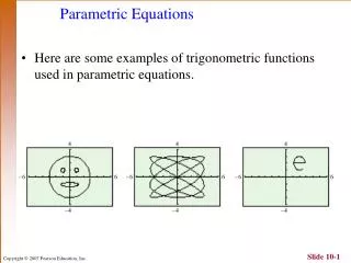
Try These Examples • See if you can also determine what the equivalent would be in y = f(x) form. • x = 2ty = 4t + 1 • x = t + 5 • y = 3t – 2 • x = 2 cos ty = 6 cos t • x = sin 4ty = cos 2t • x = 3 sin 3 ty = cos t Which one is it?
Assignment A • Lesson 6.7A • Page 440 • Exercises 1 – 9 odd 27, 29
Parametric EquationsThe Sequal Lesson 6.7B
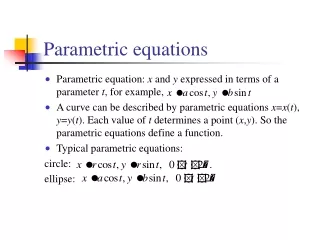
Eliminating the Parameter • Possible to represent the parametric curve with a single (x, y) equation • Example • Given x = 1 + t2 and y = 2 – t2 • Solution: • Solve 1st equation for t2 in terms of y • Substitute into 2ndequation • Result • y = 2 – (x – 1) Verify by graphing
Try It • Given x = 3 + 2 cos t and y = - 1 – 3 sin t • Hint – manipulate the equations by using Pythagorean identity sin2 t + cos2 t = 1
Path of a Projectile • Consider a projectile (such as a pumpkin) launched at a specified angle and initial velocity • Based on vector components and effects of gravity the actual path can be represented by Experiment with Pumpkin Launch Spreadsheet
Launch Another! • Graph the path of a pumpkin launched at an angle of 35° with an initial velocity of 195 ft/sec • How far did it go? • How long was it in the air?
Assignment B • Lesson 6.7B • Page 440 • Exercises 11 – 17 odd 31, 33