Staggered PRT ground clutter filtering
270 likes | 443 Views
Staggered PRT ground clutter filtering. Svetlana Bachmann November 20, 2007. Parameter q Recollect q… Motivation to change q… qGMAP… How to use GMAP with SPRT… New table q3D… Performance evaluation GCF with GMAP, TABL, q3D… Finding error & bias for power, velocity, width…

Staggered PRT ground clutter filtering
E N D
Presentation Transcript
Staggered PRT ground clutter filtering Svetlana Bachmann November 20, 2007
Parameter q Recollect q… Motivation to change q… qGMAP… How to use GMAP with SPRT… New table q3D… Performance evaluation GCF with GMAP, TABL, q3D… Finding error & bias for power, velocity, width… Examples of errors & biases… Velocity errors Mean errors… Percentage of acceptable errors… Finding a compromise… Windows… Spectral analyses Examples of mean spectra… Changes to algorithm Summary of changes… Additional possible changes…
Recollect q qis an integer. qisthe clutter width parameter used in the SPRT procedure for clutter filtering [1]. q specifies the number of spectral coefficients to be considered as the ground clutter contribution (one sided including dc). q was tabulated [1] 3 for CNR_approx < 50 dB 4 for 50 dB < CNR_approx < 70 dB 5 for 70 dB < CNR_approx < 90 dB 6 for CNR_approx > 90 dB. Reference [1] S. Torres, M. Sachidananda, D. Zrnic, “Signal design & processing techniques for WSR-88D ambiguity resolution – Part 9: Phase Coding & Staggered PRT,” NSSL Tech. report, Norman OK, 2005 (page 103, item 5)
Motivation to change q Need an adaptive qfor optimal filtering. Uniform PRT- time series Staggered PRT- Uniform PRT- spectrum Spectrum Reconstructed using Staggered PRT- TABLE GMAP
✔ Parameter q Recollect q… Motivation to change q… qGMAP… How to use GMAP with SPRT… New table q3D… Performance evaluation GCF with GMAP, TABL, q3D… Finding error & bias for power, velocity, width… Examples of errors & biases… Velocity errors Mean errors… Percentage of acceptable errors… Finding a compromise… Windows… Spectral analyses Examples of mean spectra… Changes to algorithm Summary of changes… Additional possible changes…
Spectra GCF with GMAP, TABL T1=1ms, 12 pairs, SNR=20 dB, CNR=50 dB, v=21 m s–1
Finding error & bias for P, v, w Bias: bias(P) = mean(Pi) – Po; bias(v) = mean(vi) – vo; bias(w) = mean(wi) – wo; Error: SD(P) = std(Pi); 10log(1+SD(P)/Po) SD(v) = std(vi); SD(w) = std(wi); %power P = mean(abs(Si).^2); Pi(i)=P; %velocity R1 = mean((abs(Si).^2).*... exp(j*2*pi*(0:M-1)')); v = va/pi * angle(R1); vi(i)=v; %width ln = log(P/abs(R1)) w = sqrt(2)*va/pi*... sqrt(abs(ln)).*sign(ln); wi(i)=w;
for PRT1=1 ms, dwell=60 ms, v= 4 m/s Bias: Error: q from GMAP q from the old table TABL q from the new table q3D
for PRT1=2 ms, dwell=60 ms, v= 4 m/s Bias: Error:
Performance of SPRT GCF For spectral width 4 m s–1, dwell 60 ms, PRT1 = 2 ms, q-GMAP and Blackman window Error Bias Power 〇 〇 Spectral width 〇 〇 Velocity 〇 〇 ✔ ✔ ✔ ✔ ✘ ✘ the SPRT filter fails to meet the error requirements for velocity.
✔ ✔ Parameter q Recollect q… Motivation to change q… qGMAP… How to use GMAP with SPRT… New table q3D… Performance evaluation GCF with GMAP, TABL, q3D… Finding error & bias for power, velocity, width… Examples of errors & biases… Velocity errors Mean errors… Percentage of acceptable errors… Finding a compromise… Windows… Spectral analyses Examples of mean spectra… Changes to algorithm Summary of changes… Additional possible changes…
T1, ms CNR, dB T1, ms CNR, dB Velocity: meanerror & bias (e&b) dwell = 60 ms, SNR=20 dB, v= 4 m s–1, 100 realizations for each velocity from 0 to va CNR=40 dB Error T1 = 1 ms STD_vk, k=0:va = std(vi, i=1:100) BIAS_vk, k=0:va = mean(vi, i=1:100) – vo; Mean_Error = mean(STD_vk, k=1:va) Mean_Bias = mean(BIAS_vk, k=1:va); Bias T1 = 1 ms
Velocity: meane&b dwell = 60 ms, SNR=20 dB, v= 4 m s–1, 100 realizations for each velocity from 0 to va T1 Error dwell = 60 ms ✔ ✔ ✔ ✔✗ T1, ms ✘ ✘ ✘ ✘ ✘ ✘ ✘ CNR, dB Bias dwell = 60 ms T1, ms CNR, dB
Velocity: mean e&b for different dwell times dwell = 60 ms, SNR=20 dB, v= 4 m s–1, 100 realizations for each velocity from 0 to va Error dwell = 120 ms dwell = 80 ms dwell = 100 ms dwell = 60 ms T1, ms CNR, dB Bias dwell = 120 ms dwell = 80 ms dwell = 100 ms dwell = 60 ms T1, ms CNR, dB
Velocity: mean e&b for different spectral widths dwell ~ 60 ms, SNR=20 dB, v= 4 m s–1, 100 realizations for each velocity from 0 to va Error v = 4 m s–1 3½ m s–1 2½ m s–1 3 m s–1 T1, ms CNR, dB Bias v = 4 m s–1 3½ m s–1 2½ m s–1 3 m s–1 T1, ms CNR, dB
T1, ms CNR, dB T1, ms CNR, dB Velocity: % of acceptable e&b dwell = 60 ms, SNR=20 dB, v= 4 m s–1, 100 realizations for each velocity from 0 to va CNR=40 dB Accept. Error T1 = 1 ms STD_vk, k=0:va = std(vi, i=1:100) BIAS_vk, k=0:va = mean(vi, i=1:100) – vo; Mean_Error = mean(STD_vk, k=0:va) Mean_Bias = mean(BIAS_vk, k=0:va); e = STD_v(abs(STD_v) < 2); Accept_Error = length(e)/length(STD_v); b = BIAS_v(abs(BIAS_v) < 2); Accept_Bias = length(b)/length(BIAS_v); Accept. Bias T1 = 1 ms
Velocity: % of acceptable e&b dwell = 60 ms, SNR=20 dB, v= 4 m s–1, 100 realizations for each velocity from 0 to va Accept. Error T1, ms CNR, dB Accept. Bias T1, ms CNR, dB
Velocity: % of acceptable e&b fordifferent dwell times dwell ~ 60 ms, SNR=20 dB, v= 4 m s–1, 100 realizations for each velocity from 0 to va Accept. Error dwell = 120 ms dwell = 80 ms dwell = 100 ms dwell = 60 ms T1, ms CNR, dB Accept. Bias dwell = 120 ms dwell = 80 ms dwell = 100 ms dwell = 60 ms T1, ms CNR, dB
Velocity: % of acceptable e&b fordifferent spectral widths dwell ~ 60 ms, SNR=20 dB, v= 4 m s–1, 100 realizations for each velocity from 0 to va Accept. Error v = 4 m s–1 3½ m s–1 2½ m s–1 3 m s–1 T1, ms CNR, dB Accept. Bias v = 4 m s–1 3½ m s–1 2½ m s–1 3 m s–1 T1, ms CNR, dB
120 ms 80 ms 100 ms 60 ms T1, ms 4 m s–1 3½ 3 2½ 2½ 3 3 120 ms 80 ms 100 ms 60 ms CNR, dB T1, ms T1, ms 120 ms 80 ms 100 ms 60 ms T1, ms CNR, dB CNR, dB CNR, dB 4 m s–1 v = 4 3½ 3½ 2½ 2½ 3 3 120 ms 80 ms 100 ms 60 ms T1, ms T1, ms T1, ms CNR, dB CNR, dB CNR, dB Velocity: mean e&b and % of acceptable e&b v= 4 m s–1 dwell = 60 ms Mean error Accept. Error Mean bias Accept. bias
Velocity e&b: a compromise SNR = 20 dB, v = 3 m/s, dwell 80 ms
✔ ✔ Parameter q Recollect q… Motivation to change q… qGMAP… How to use GMAP with SPRT… New table q3D… Performance evaluation GCF with GMAP, TABL, q3D… Finding error & bias for power, velocity, width… Examples of errors & biases… Velocity errors Mean errors… Percentage of acceptable errors… Finding a compromise… Windows… Spectral analyses Examples of mean spectra… Changes to algorithm Summary of changes… Additional possible changes… ✔ ✔
Changes to algorithm Step pre-compute: Ignore the power loss correction factor, instead normalize the window Step 2. Apply normalized window – Blackman (?) Step 4. • If q3D:do not divide by N when computing CNR_approx: CNR_aprox = sum(abs([Vr(1), Vr(2), Vr(end)].^2)).*25/4./(N*NoiseLevel); replace “power” with “amplitude” in the comment; • If qGMAP: this step can be omitted. Step 5. Clutter width parameter is determined either from q3D or using GMAP • If q3D: estimate CNR_approx, Np, and va and choose q from table table q3D<30x50x10>, where i_CNRdB 1:2:60, i_Mp 10:59, i_va 20:5:65 x = round((CNRdb_aprox/2)); if x<1 x=1; end; if x>30 x=30; end; y = round((Np-9)); if y<1 y=1; end; if y>50 y=50; end; z = round(va/5-3); if z<1 z=1; end; if z>10 z=10; end; q=round(q3D(x, y, z)); • If qGMAP: modify GMAP to return number of coefficient identified as clutter; take the 5th of the Doppler spectrum (containing the main clutter replica and whichever weather replica); initialize GMAP for spectra with va/5; pass the 5th of Doppler spectrum to GMAP; use the number of coefficients identified as clutter to estimate q. Step 8. Add “diag” in front of the clutter filter matrices If1, If2 Step 11. Remove “1/N” from autocorrelation formula Step 12. Choose symmetric window of samples around the rounded to the nearest sample velocity estimate k0: k1=k0 – floor(M/4)+1 ; k2=k0 + floor(M/4) Step 16. Same as in step 12. Steps 12, 13, and 16 must be changed to accommodate odd pairs. Step 17. Replace “6.37” with “6.27” Acknowledgements: David Warde, Sebastian Torres, Dusan Zrnic ✔ ✔ ✔
✔ ✔ Parameter q Recollect q… Motivation to change q… qGMAP… How to use GMAP with SPRT… New table q3D… Performance evaluation GCF with GMAP, TABL, q3D… Finding error & bias for power, velocity, width… Examples of errors & biases… Velocity errors Mean errors… Percentage of acceptable errors… Finding a compromise… Windows… Spectral analyses Examples of mean spectra… Changes to algorithm Summary of changes… Additional possible changes… ✔ ✔ ✔