Download
1 / 24
240 likes | 381 Views
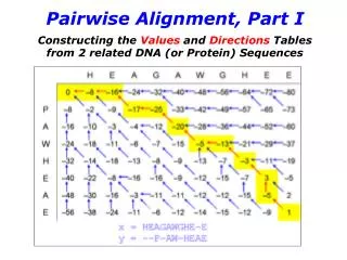
Pairwise Alignment, Part I. Constructing the Values and Directions Tables from 2 related DNA (or Protein) Sequences. Pairwise Alignment of DNA (or Amino Acid) Sequences.

E N D
Pairwise Alignment, Part I Constructing the Values and Directions Tables from 2 related DNA (or Protein) Sequences
Pairwise Alignment of DNA (or Amino Acid) Sequences Given a pair of DNA gene sequences – each from a different species – one way to determine how related the species are is to calculate the degree of homology that the sequences share. We assume that the more similar the sequences, the more closely related the species are. ATCTGATG TGCATAC The problem is complicated because, in the course of evolution, bases may have been inserted into or deleted from the sequence. The algorithm therefore must also take into account how best to align the two sequences for comparison. We are going to use a technique based on the LCS – Longest Common Subsequence– algorithm. The first part of the algorithm constructs a TABLE of DATA, similar to a multiplication table. However, instead of numbers in the headers (along the top and left sides), we place the letters of each DNA sequence. Before we write a Java program (in the subsequent lesson), we will model this algorithm in an Excel spreadsheet.
Type the labels Seq 1 and Seq 2 in A1 and A2. Center- or Right-Align A1:A2. The actual sequences themselves go in B1 and B2. Left-Align B1:B2. It’s best to use the Paste Special Values command for the sequences so as not to overwrite the formatting.
The number series 1-10 go in the horizontal range D8:M8 and the vertical range A11:A20. The hard-coded number 1 goes in the first cell of each range (D8 and A11). The formula ’Previous-Cell-Reference’ + 1 can be copied to the remaining cells, as shown below. Use Ctrl+~ to toggle in and out of Formula Mode.
Next we fill in the HEADERrow and column with the individual letters of Sequences 1 and 2, respectively. We do this using formulas…
Using the horizontal and vertical 1-10 series, we can EXTRACT individual letters from each of the sequences with the MID() function. The 1stargument is the cell address of the sequence. We use a $ to absolute cell reference either the column (Seq 1) or the row (Seq 2) so that each formula can be copied across or down, respectively. The 2nd argument is the position of the character we want to extract. The 3rd argument is the number of characters we want to extract, in this case 1. This technique allows us to paste different sequences into cells B1 or B2 without having to manually enter each character into the header cells of the table. Note that the formulas con-veniently place blanks in the cells beyond the last letter of each sequence.
Below is the pseudo-code for generating the table data for the LCS algorithm. The algorithm uses a 2-D array, whose cells are referenced by row and column (r,c) as depicted in the grid above. The variable i refers to the rows, The variable j refers to the columns. In the pseudo-code, c[i, j] is the value that is placed in the cell ( r=i, c=j )
We first initialize the cells in the row and column next to the headers to zeroes.
Rather than hard-code each zero, we hard-code only the zero in C10. We use formulas in the other cells so that zeroes appear only in columns and rows where there are header letters. Copy the formula in D10 across and the formula in C11 down . Note again that these formulas conveniently place blanks (rather than zeroes) in the cells beyond the last letter of each sequence. If we paste sequences of different lengths into B1 or B2, we will not have to reprogram these cells.
We now create a single formula in D11 that we will copy to every other data cell in the table. The formula will use the if … else if … else conditional statements on lines 9-16.
Lines 9-10: If the two bases in the headers are the SAME, then the value of the cell that their row/column combination intersects is 1 plus the value in the cell along the diagonal in the previousrow and column, i.e. the value to the cell’s top left. The 2 bases are the same for cell(2,1), i.e. T = T. The value in this cell is calculated by adding 1 to the value in the diagonally placed cell (1,0) in the previous row & column. +1 VALUE in cell (2,1) VALUE in cell(1,0) + 1
Lines 12-13,15: If the two bases in the headers are DIFFERENT, then the value of the cell that their row/column combination intersects is the larger of the values in the previous row or the previous column, i.e. the values above and to the left. The 2 bases are different for cell(2,2), i.e. G <> T. The value in this cell is calculated by taking the larger of the 2 values in the cells above and to the left. VALUE in cell (2,2) MAX(cell(1,2), cell(2,1)) above left
When we combine these two conditions, we end up with the formula for D11 below. Copy this formula to all the cells in the table.
A problem emerges after copying the D11 formula to the rest of the table’s data cells. We really want the cells in columns 7-10 and rows8-10 to be blank. We can accomplish this with an extra IF condition prepended to our formula:
The 1st Data Table is now complete and should look like the image below.
Constructing the Directions Table The 2nd Data Table will consist of Direction data indicating one of the 3 neighbor cells (left, above, diagonal) relative to the current cell. For example, if 2 bases are the same, the arrow will point back to the diagonal cell. If the 2 bases are different, we will use either the or arrows to indicate the cell above or to the left, depending upon which one was the largest. This information will allow us to backtrack and reconstruct the entire path traveled in calculating a cell’s value. To start, delete the other empty worksheets in your document and RENAME your remaining worksheet Values.
Make an exact copy of the worksheet by right-clicking on the worksheet label (Values). Select Move or Copy from the pop-up menu. In the Move or Copy Dialog: (1) Select (move to end) (2) CheckCreate a copy Rename the duplicate worksheet: Directions
From Excel’s main menu, select the Viewmenu (1) . Select New Window(2), then Arrange All(3). In the Arrange Windows dialog, select Vertical(4). You should now see 2 windows side-by-side. Select the Values worksheet in one and the Directions worksheet in the other.
Every cell in the Directions table will mirror its counterpart in the Values table, using a formula containing just the cell reference / address of the Values table cell. Create a new formula in cell A1 of the Directions table by entering the = sign. Then click on cell A1 in the Values table. The formula =Values!A1 will appear in cell A1 of the Directions table. In the Directions table, use the Paste Special command to copy only the FORMULA part of cell A1 to the ranges A1:B2, A11:C20, D8:M10, and C10. This way, each cell will keep its unique formatting.
We will now modify the formula in cell D11 in the Directions table For the part of the formula that checks whether the 2 bases are the same, simply substitute “\” into the true part of the IF statement. We will replace the MAX() function in the false part of the IF statement, because the MAX() function does not tell us which cell (left or above) was used. We therefore use another IF statement to check whether the value in the cell above (D10) is >= to the value in the cell to the left (C11). If so, we place “↑“ in the cell. If not, we place “←” in the cell. NOTE: We need to check the D10 and C11 cells in the Values table, since the corresponding cells in the Directions table will be filled with arrows, not numbers. You can now copy the formula in D11 to the 99 other data cells in the Directions table, the range D11:M20. Arrow Keys: From the Windows Start Menu, select Accessories System Tools Character Map tool to access the Left Arrow (“←” Unicode 2190) and Up Arrow (“↑“ Unicode 2191) characters. Because there is no easy way to depict a diagonal arrow, we’ll use the Backslash character (“\” Unicode 005C / decimal 92) in its place. [Or just copy them from here].
The completed Directions table should appear as in the image below.
Below is a View of the 2 Completed tables for the Original Test Sequences.
Below is a View of the 2 Completed tables for the Original Test Sequences, where Seq 1 and Seq 2 have exchangedplaces. Use Paste Special → Values to preserve cell formatting. Make the change in the Values table; the Directions table will automatically reflect the changes.