Download
1 / 19
190 likes | 228 Views
Learn about the various methods for weighting criteria in decision-making processes, including SMART and AHP, and how to handle incomplete ordinal preference information effectively.

E N D
RICH - Rank Inclusion in Criteria Hierarchies Ahti Salo and Antti Punkka Systems Analysis Laboratory Helsinki University of Technology http://www.sal.hut.fi/
Multi-attribute weighting Subcontractor Schedule(a1) Quality of work (a2) Overall cost (a3) References (a4) Possibility of changes (a5) Large firm (x1) Small entrepreneur (x2) Medium-sized firm (x3)
Weighting methods • Tradeoff method • has a sound theoretical foundation • requires continuous measurement scales • may be difficult in practice • Ratio-based methods • popular even though the theoretical foundation • SMART (Edwards 1977) • AHP (Saaty 1980) • Ordinal judgements • ask the DM to rank the attributes in terms of importance • derive a representative weight vector from this ranking • e.g., SMARTER (Edwards and Barron 1994), rank sum weights
Incomplete information • Complete information may be hard to acquire • alternatives and their impacts? • relative importance of attributes? • Examples • assessment of environmental impacts • cost of information acquisition • inability to consult all stakeholders • fluctuating preferences • What can be concluded on the basis of available information? • parametric uncertainties covered • structural uncertainties excluded
Analysis of ordinal preference statements • Earlier approaches to the analysis of ordinal information • ask the DM to rank the attributes in terms of importance • derive a representative weight vector from the ranking • e.g., SMARTER (Edwards and Barron 1994), rank sum weights • Incomplete ordinal preference information • the DM(s) may be unable to rank the attributes • statements on contentious issues may be difficult • ”which is more important - economy or environmental impacts” • equal weights sometimes used as an approximation • Incomplete ordinal information in RICH • associate a set of possible rankings with a given set of attributes • these statements define possibly non-convex feasible regions
Notation • I is a set of attributes, J a set of rank numbers • r a rankingis a mapping from attributes to • r(ai) is the rank of attribute i • Compatible rank orders • Feasible region for a given rank order r • Feasible region for rank orders compatible with the sets I and J
Preference elicitation - example 2 • The most important attribute is either a1 or a2 • This leads to attribute set I={a1,a2} and rank set J={1} • Compatible rank orders are (a1,a2,a3), (a1,a3,a2), (a2,a1,a3), (a2,a3,a1) • Feasible region not convex
Preference elicitation - example 1 • Attributes a1 and a2 are the two most important attributes • This leads to attribute set I={a1,a2} and rank set J={1,2} • Compatible rank orders are (a1,a2,a3) and (a2,a1,a3) • Sp(I)=S(I,{1,…,p})
Feasible regions • Feasible region associated with certain I and J is equal to that of complement of I and complement of J • If there are more ranks in J than attributes in I, the feasible region gets smaller when attributes are added to I • If there are less ranks in J than attributes in I, the feasible region gets larger when attributes are added to I
Feasible regions • When there are less ranks in J than attributes in I, the feasible region gets smaller, when ranks are added to J • When there are more ranks in J than attributes in I, the feasible region gets bigger, when ranks are added to I
Measure for the feasible region • Measure of completeness • compares the number of compatible rank orders to the total number of rank orders
Decision criteria • Pairwise dominance • Maximax • alternative with greatest maximum value • Maximin • alternative with greatest minimum value • Minimax regret • alternative with smallest possible difference to greatest maximum value • Central values • alternative with greatest sum of maximum and minimum value
Application of decision criteria • What concluded when dominance results do not hold? • extrapolate from the available preference information • develop recommendations through alternative decision criteria • analogues include "expected value" etc. • Possible loss of value • what may be lost by terminating the analysis early? • indicates sensitivities in parameter values • can be mapped back to single-attribute scores • helps in assessing the value of additional information
Computational convergence • Questions • how effective are this kind of statements? • which decision rules are best? • Randomly generated problems • n=5,7,10 attributes; m=5,10,15 alternatives • 3 different preference statements • A. DM knows the most important attribute • B. DM knows two most important attributes • C. DM knows a set of 3 attributes, which contains 2 most important • statements were compared to equal weights and complete rank orders • efficiency was studied using central values (appeared to be best) • 5000 problem instances • values computed in extreme points
Results • Statements improve performance in relation to equal weights • Rank order is better than the studied statements • Statement B gives the best results • the feasible region is smallest
Conclusion • PRIME characteristics • acknowledgement of uncertainties • maintenance of consistencies • alternative elicitation processes • intermediate guidance through decision rules • PRIME Decisions • full-fledged computer implementation • interactive decision support • downloadable at http://www.hut.fi/Units/SAL/Downloadables/
References Salo, A. and R.P. Hämäläinen, "Preference Programming through Approximate Ratio Comparisons," European Journal of Operational Research 82 (1995) 458-475. Salo, A. ja R.P. Hämäläinen, "Preference Assessment by Imprecise Ratio Statements," Operations Research 40/6 (1992) 1053-1061. Salo, A., "Interactive Decision Aiding for Group Decision Support," European Journal of Operational Research 84 (1995) 134-149. R.P. Hämäläinen and M. Pöyhönen, "On-line group decision support by preference programming in traffic planning,"Group Decision and Negotiation 5 (1996) 485-500. Gustafsson, J., Salo, A. and Gustafsson, T., “Prime Decisions: An Interactive Tool for Value Tree Analysis,” In Köksalan, M. and Zionts, S (Eds.), Multiple Criteria Decision Making in the New Millenium, Lecture Notes in Economics and Mathematical Systems, vol. 507, pp. 165-176, Springer-Verlag, Berlin. Mustajoki, J., Hämäläinen, R. P. and Salo, A., “Decision support by interval SMART/SWING - methods to incorporate uncertainty into multiattribute analysis,” Systems Analysis Laboratory, Helsinki University of Technology, Manuscript. Salo, A. and Hämäläinen, R. P., “Preference Ratios in Multiattribute Evaluation (PRIME) - Elicitation and Decision Procedures under Incomplete Information,” IEEE Transactions on Systems, Man, and Cybernetics (to appear).