Pincascia Lavertezzo 44km 2

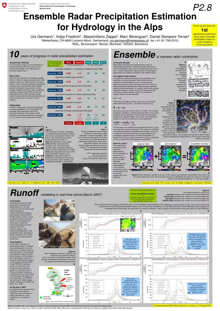
1. FOEN river gauges PincasciaLavertezzo44km2 Verzasca Lavertezzo186km2 automaticraingauges 10 km FOEN = Swiss Federal Office for the Environment Figure 2: Detailed knowledge of the radar error structure (e.g. variability of Z-R relation) and stochastic variations belong to the repertoire of the radar ensemble. Bias Scatter POD FAR ETS in terms of water amounts for 0.3mm daily rainfall Factor Factor % % % 0.76 0.39 0.89 0.58 0.38 2.0 3.0 2.5 2.0 2.5 73 87 84 75 89 30 8 8 14 34 57 40 39 53 62 Summer 2001 Summer 1997 Summer 1998 Summer 1999 Summer 2004 Table 1:Results of systematic large-sample verification of operational radar estimates of surface recipitation rates for the whole of Switzerland. Of course, one can find even better agreement if subjectively selecting the "nice cases". We prefer, however, the honest objective approach taking into account all days of a long period and gauges spread over the whole country!POD = probability of detectionFAR = false alarm ratioETS = equitable threat score(Joliffe and Stephenson, Wiley, 2003) Verzasca river, 186km2, Southern Alps Radar driven runoff (yellow, blue, red, black) overestimate observed runoff (green). Raingauge runoff (pink) is close to observed runoff. Radar (blue, red, yellow, black) captures well the observed runoff (green), and clearly beats raingauges (pink). Figure 5:Map of Verzasca catchment (186km2) and Pincascia sub-catchment (44km2). In Fig. 3 Verzasca is indicated in yellow. River gauges are indicated by red arrows. Automatic rain gauges are indicated by green circles. 2864m Raingauge driven runoff (pink) often underestimates observed runoff (green) because raingauges miss strong orographic precipitation over the mountainous regions with bad raingauge coverage. 193m P2.8 Ensemble Radar Precipitation Estimation for Hydrology in the Alps Urs Germann1, Katja Friedrich1, Massimiliano Zappa2, Marc Berenguer3, Daniel Sempere-Torres41MeteoSwiss, CH-6605 Locarno-Monti, Switzerland, urs.germann@meteoswiss.ch, fax +41-91-756-2310; 2WSL, Birmensdorf; 3McGill, Montréal; 4GRAHI, Barcelona As far as we know the 1stoperational experiment using radar ensemble precipitation fields for runoff modelling in the mountains. 10 Ensemble years of progress in radar precipitation estimation to express radar uncertainty 3 radars, 58 gauges, all (!!) days between May and October In the past decadeMeteoSwiss developed and implemented a series of sophisticated algorithms to obtain best radar estimates of surface precipitation rates over all of Switzerland (see to the left). In spite of significants improvements, for hydrological applications the residual uncertainty is still relatively large. Of particular difficultyin a mountainous region are the elimination of ground echoes and the correction of errors caused by shielding of the radar beam by mountain ranges (Fig. 1). Much effortwent into the optimization of hardware stability (Cavalli, 1999) and data processing of the radar network (Joss et al, 1998; Germann and Joss, 2004) in order to obtain quantitative precipitation estimates that meet both the meteorologist's and the hydrologist's requirements. A large-sample comparison between radar precipitation estimates (radar product RAIN) and ground observations from a high-resolution gauge network reveals distinct improvements achieved by the modifications of the past 10 years (Table 1). NowcastingIn 2003 a radar-based nowcasting application for heavy precipitation was implemented. An automatic alert message is sent to the forecaster whenever accumulated rainfall exceeds a pre-defined threshold for periods of 3, 6, 12 and 24 hours (radar product NASS). automatic calibration + monitoring of hardware since 1993 An elegant novel solutionto express the residual uncertainty is the generation of an ensemble of radar precipitation fields using stochastic simulation and knowledge of errors. In a first step we determine the mean μand covariance matrix C of errors in radar precipitation estimates by comparing radar estimates against ground observations of a gauge network with average separation distance of 10km. Second, we decompose the (symmetric, positive definite) matrix C by Cholesky or Singular-Value (SV) decomposition LLT = C Third, we pre-multiply a random zero-mean unit-variance white-noise vector εiwith L, and add the mean error μ δi = μ+ Lεi where δi, μand εi are vectors and L is a matrix. The resulting perturbation field δi is correlated Gaussian with correct means, variances and covariances. Fourth we add the perturbation field δi to the original field R0. This is done in the logarithmic domain as most of the radar errors are multiplicative log(R'i) = log(R0) + δi The first term is the deterministic component (fixed for a given time step), the second is stochastic. The result is an ensemble of perturbed precipitation fields R'i each member i of which is in agreement with the deterministic component R0and our knowledge of spatial structure of radar uncertainties. To impose the observed temporal structure of radar uncertainties we use a 2-parameter autoregressive model AR(2). implement visibility map correction improve operational ground echo elimination implement correction for vertical reflectivity profile implement global bias correction Figure 3:A prototype ensemble generator was implemented for a 2800km2 test catchment in Southern Switzerland, north of Lema radar. 31 gauges (white squares) are used to determine the radar error mean μ and covariance matrix C of the 700 2km-catchment- local bias correction (training with 2003 data) 1.00 1.7* 90 15 63 Summer 2004 *1.4 for subjective data set missed water=2% false water=1‰ probabilistic deterministic stochastic Figure 1:The challenge in the Alps: combination of shielding and ground clutter inhibits a direct view on precipitation close to the ground. The 4 panels show vertical cross-sections from 0-6km of (top) scan geometry of Lema radar, (2nd) intensity of ground clutter averaged over 1 hour during fine weather (clutter elimination algorithm turned off; red corresponds to >21 dBZ), (3rd) pixels frequently eliminated by the clutter elimination algorithm, and (bottom) two-day accumulation of precipitation illustrating the convolution of scan geometry, beam shielding and orographic precipitation mechanisms. pixels (pink crosses). Greyshading corresponds to terrain height. Runoff modelling was implemented for the Verzasca catchment (yellow), see below. Note on μ and CThe mean μ and covariance matrix C are first determined for 24-hour periods, as most of the 31 gauges shown in Fig. 3 are daily reporting. μ and C are then extrapolated to 1-hour periods using linear scaling as observed for the 8 automatic gauges with 10min resolution. perturbation ensemble member original field + = Figure 4: Each ensemble member is the sum of the original radar field plus a perturbation field, which has the correct space-time mean and covariance structure as defined by the radar error structure. The figure shows one ensemble member for a 1-hour accumulation. Germann et al., 2006, Q. J. R. Meteorol. Soc.,132, 1669-1692 Germann et al, 2006, Proc. Europ. Conf. on Radar in Meteorol. and Hydrol., 559-562. Photo Alo Zanetta Monte Lema radar, 1625m Runoff The four examples shown below are a honest representative sampleof all results obtained so far, and include both “nice” and “bad” cases (from a radar scientist’s point of view). Figure 6:First results obtained in real-time for(top-left) Pincascia river, model run at 18 June 0000 UTC,(bottom-left) Verzasca river, model run at 18 June 0000 UTC,(top-right) Pincascia river, model run at 25 June 0000 UTC,(bottom-right) Verzasca river, model run at 25 June 0000 UTC.Runoff observed at river gauge is indicated in green. Runoff modelled using precipitation from raingauge as input is shown in pink; other colours show runoff calculated with radar ensemble precipitation fields as input. No post-facto calibration or tuning. Model parameters were calibrated using raingauge and rivergauge data of past events. No radar data was used for calibration. There is space for improvements using also radar for model calibration. modelling in real-time (since March 2007) A prototypeensemble generator for radar precipitation estimation was implemented in a real-time context as part of the Mesoscale Alpine Programme hydrometeorological forecast demonstration project MAP D-PHASE (Rotach, 2004) and the European concerted research action on the propagation of uncertainty in advanced hydrometeorological forecast systems COST-731 (cost731.bafg.de). The operational MeteoSwiss radar precipitation fields described in detail in Germann et al. (2006) are taken as the deterministic component. Perturbationsfor the radar ensemble are generated by means of singular value decomposition of the full radar error covariance matrix as described above. The ensemble of precipitation field time series, which consists of 25 members, is then assimilated in real-time in the semi-distributed precipitation-runoff-evapotranspiration-HRU model PREVAH to calculate runoff of the Verzasca and Pincascia rivers at the river gauges in Lavertezzo (Fig. 5). These are steep mountainous catchments prone to flash floods in the Southern Swiss Alps. For more information on PREVAH see Gurtz et al. (1999), Zappa (2003), Wöhling et al. (2006) and Ranzi et al. (2007). At the end of 2007we hopefully have enough events to perform a first objective evaluation of the usefulness of radar ensembles for runoff modelling in a mountainous region. 13 18 Radar, 15 June, 14-15UTCsame region + colors as Fig. 4 hours hours With present implementation the ensemble mean (blue) is larger than the determinstic (yellow) because perturbation is symmetric in log. This can be fixed by adapting μwhich is currently being tested. hours hours First presented at AMS Radar Conference in Cairns, 6-10 August 2007. Thanks to Ufficio dei corsi d’acqua of Canton Ticino and Swiss Federal Office for the Environment for river and rain gauge data. Special thanks to Jürg Joss, Remo Cavalli, Gianmario Galli, Marco Boscacci and Alessandro Hering for continuous support and many fruitful discussions.