Binary Trees (7.3)
Binary Trees (7.3). CSE 2011 Winter 2011. Binary Trees. A tree in which each node can have at most two children. The depth of an “average” binary tree is considerably smaller than N. In the worst case, the depth can be as large as N – 1. Generic binary tree. Worst-case binary tree.

Binary Trees (7.3)
E N D
Presentation Transcript
Binary Trees (7.3) CSE 2011 Winter 2011
Binary Trees • A tree in which each node can have at most two children. • The depth of an “average” binary tree is considerably smaller than N. In the worst case, the depth can be as large as N – 1. Generic binary tree Worst-casebinary tree
Decision Tree • Binary tree associated with a decision process • internal nodes: questions with yes/no answer • external nodes: decisions • Example: dining decision Want a fast meal? No Yes How about coffee? On expense account? Yes No Yes No Starbucks Spike’s Al Forno Café Paragon
+ 2 - 3 b a 1 Arithmetic Expression Tree • Binary tree associated with an arithmetic expression • internal nodes: operators • external nodes: operands • Example: arithmetic expression tree for the expression (2 (a - 1) + (3 b))
The BinaryTree ADT extends the Tree ADT, i.e., it inherits all the methods of the Tree ADT Additional methods: position left(p) position right(p) boolean hasLeft(p) boolean hasRight(p) Update methods may be defined by data structures implementing the BinaryTree ADT BinaryTree ADT Trees
Implementing Binary Trees • Arrays? • Discussed later • Linked structure?
Linked Structure of Binary Trees class BinaryNode { Object element BinaryNode left; BinaryNode right; BinaryNode parent; }
D C A B E Linked Structure of Binary Trees (2) • A node is represented by an object storing • Element • Parent node • Left child node • Right child node B A D C E
Binary Tree Traversal • Preorder (node, left, right) • Postorder (left, right, node) • Inorder (left, node, right)
Preorder Traversal: Example • Preorder traversal • node, left, right • prefix expression • + + a * b c * + * d e f g
Postorder Traversal: Example • Postorder traversal • left, right, node • postfix expression • a b c * + d e * f + g * +
Inorder Traversal: Example • Inorder traversal • left, node, right • infix expression • a + b * c + d * e + f * g
A binary trees is proper if each node has either zero or two children. Level: depth The root is at level 0 Level d has at most 2d nodes Notation: n number of nodes e number of external (leaf) nodes i number of internal nodes h height n = e + i e = i +1 h+1 e 2h n =2e -1 h i 2h – 1 2h+1 n 2h+1– 1 log2e h e – 1 log2 (i +1) h i log2 (n +1)-1 h (n -1)/2 Properties of Proper Binary Trees
Level: depth The root is at level 0 Level d has at most 2d nodes Notation: n number of nodes e number of external (leaf) nodes i number of internal nodes h height h+1 n 2h+1– 1 1 e 2h h i 2h – 1 log2 (n +1)-1 h n -1 Properties of (General) Binary Trees
Array-Based Implementation Nodes are stored in an array. A … B D C E F J G H 1 2 3 • Let rank(v) be defined as follows: • rank(root) = 1 • if v is the left child of parent(v), rank(v) = 2 *rank(parent(v)) • if v is the right child of parent(v), rank(v) = 2 *rank(parent(v)) + 1 4 5 6 7 10 11 Trees 16
Array Implementation of Binary Trees Each node v is stored at index i defined as follows: If v is the root, i = 1 The left child of v is in position 2i The right child of v is in position 2i + 1 The parent of v is in position ??? 17
Space Analysis of Array Implementation n: number of nodes of binary tree T pM: index of the rightmost leaf of the corresponding full binary tree (or size of the full tree) N: size of the array needed for storing T; N = pM + 1 Best-case scenario: balanced, full binary tree pM = n Worst case scenario: unbalanced tree Height h = n – 1 Size of the corresponding full tree: pM = 2h+1– 1= 2n – 1 N = 2n Space usage: O(2n) 18
Arrays versus Linked Structure Linked lists Slower operations due to pointer manipulations Use less space if the tree is unbalanced AVL trees: rotation (restructuring) code is simple Arrays Faster operations Use less space if the tree is balanced (no pointers) AVL trees: rotation (restructuring) code is complex 19
Next time … • Binary Search Trees (10.1)