Download
1 / 43
460 likes | 556 Views
Dive into models of common-mode vs. differential currents, principles of switch power supply, and maximizing EMC emission mitigation strategies. Learn how current probes measure emissions & more in this enlightening lecture.

E N D
Radiated Emissions and Susceptibility Common-Mode vs. Differential Mode Currents Emission Models for Wires and PCB Lands Use of current probe to measure common-mode currents Use of common-mode choke to block conducted emissions Principle of operation of switching power supply Use of current probe as diagnostic tool in EMC Lecture 12 Radiated Emissions
Common-Mode and Differential Mode Currents in Parallel Conductors I1 Ic ID ID Ic I2 Lecture 12 Radiated Emissions
Why do we care about common-mode and differential-mode currents? Lecture 12 Radiated Emissions
Differential-mode and Common-mode currents in parallel conductors Lecture 12 Radiated Emissions
Net E field is superposition of the far fields set up by both wires, treated as Hertzian dipoles Eθ = Eθ,1 + Eθ,2 Lecture 12 Radiated Emissions
We may model a single wire of length L (L << λ) carrying sinusoidal (phasor) current I1 as a Hertzian Dipole. Therefore the phasor representation of the radiated E field at a distance of “r1” at an angle of “θ” w.r.t. the wire axis due to the sinusoidal current “I1” flowing in Wire #1 of length “L” is given by: Lecture 12 Radiated Emissions
Differential Mode Emission Model: The currents “ID” flow in oppositedirections as shown below. The model can be simplified considerably if we are interested in the maximum emission that would be picked up from two electrically short conductors of length L (L << λo) that are separated by distance “s”, where our observation point is oriented “broadside” to the two conductors (θ = π/2 radians), in order to receive the maximum emission, at an observation point that is a distance d from the center of the conductors. Lecture 12 Radiated Emissions
(mks units assumed) V/m Note that the magnitude of the unintentionally radiated E field is directly proportional to wire length L, the square of the current frequency “f”,loop area “L*s”, and the current magnitude, and falls off as 1/d. Thus differential-mode currents with high frequency components (shorter pulse widths with shorter rise and fall times) will result in stronger unwanted emissions. Also, keeping the loop area “L*s” small and the current levels low helps reduce these emissions. Lecture 12 Radiated Emissions
Common-Mode Emission Model: Now the currents “IC” flow in the same direction as shown below. The model can be simplified considerably if we are interested in the maximum emission that would be picked up from two electrically short conductors of length L (L << λo) that are separated by distance “s”, where our observation point is oriented “broadside” to the two conductors (θ = π/2 radians), in order to receive the maximum emission, at an observation point that is a distance d from the center of the conductors. Lecture 12 Radiated Emissions
V/m (mks units assumed) Note that the magnitude of the unintentionally radiated E field is directly proportional to the line length L, the current frequency “f”, and the current magnitude, and it falls off as 1/d. Thus common-mode currents with higher frequency components (shorter pulse widths with shorter rise and fall times will result in stronger unwanted emissions.) Also, reducing the current level and line length will decrease unwanted emissions. Lecture 12 Radiated Emissions
Example of estimating the net maximum far-field strength from two parallel wires I1 = -20 mA @ 200 MHz 1.5 cm I2 = 10 mA @ 200 MHz 0.5 m Find the magnitude of the total maximum far field electric field strength in dBμV/m at a distance of 15 meters from the two wires that carry the 200 MHz sinusoidal currents shown. Solution: IC = (-20+10)/2 = -5 mA ID = (-20-10)/2 = -15 mA Lecture 12 Radiated Emissions
15 mA 5 mA 15 mA 5 mA ED EC Note: Etot = ED-EC Lecture 12 Radiated Emissions
Use of current probe Lecture 12 Radiated Emissions
Current Probe responds to common-mode currents while rejecting differential-mode currents • Current probe responds to the NET ac current flowing through it. Thus, if both conductors are enclosed by the toroidal core of the current probe, the net current is: I1 + I2 = (Ic + Id) + (Ic – Id) = 2Ic • Only the common-mode current is measured! • The only way to measure differential mode current is to put one conductor at a time in the current probe! Lecture 12 Radiated Emissions
Current Probe Transfer Impedance • Definition: The (frequency-dependent) transfer impedance ZT of a current probe is the ratio of the phasor voltage at its output (V) to the phasor current that it is measuring (I) • ZT = V / I • |ZT| = | V | / | I | • |ZT|dB = | V |dBμV - | I |dBμA • | I |dBμA = | V |dBμV - |ZT|dB Lecture 12 Radiated Emissions
Typical current probe transfer impedance curve (ZdB vs frequency) Lecture 12 Radiated Emissions
Use of the Current Probe as a diagnostic tool in EMC • Our text points out (p. 522) that the current probe can be a very important diagnostic tool in EMC. • When prototyping a new product, it is a simple matter to measure the net currents on the cables extending from the product, and taking steps to reduce these net (common-mode) currents by adding toroidal common mode chokes, etc. • This is far more efficient than scheduling time on a full-blown expensive anechoic chamber test. • This gives the same information, but in real time! • An empirical calibration chart can be made that relates net cable current to various regulatory RF emission limits. Lecture 12 Radiated Emissions
Current Probe Example Lecture 12 Radiated Emissions
Simple Susceptibility Model • We have developed simple common-mode and differential mode radiation models from electrically short circuits which let us predict the maximum radiated RF E field magnitude at a specified distance from the radiating circuit. • We now turn our attention to the other side of the coin: here we shall develop a simple susceptibility model that lets us predict the voltage and current induced in an electrically short circuit in the presence of a radiating RF E field of specified magnitude and orientation relative to the plane of the circuit. Lecture 12 Radiated Emissions
Modeling 2-conductor line in presence of interfering EM field: Only Ey = ET and –Hz = HN field components affect the 2-conductor line. Faraday’s Law of induction may be used to find the voltage per unit length (Vs) that is induced in the loop due to the time-varying normal HN field component. The induced current per unit length (Is) flowing down through the line capacitance “CΔx”. Which is due to the applied time-varying ET field component can be found from the formula for current through a capacitor (iC = CdV/dt) where C = CΔx and Lecture 12 Radiated Emissions
Simplified Lumped Parameter Model for line length Δx << λ (series inductance and shunt capacitance can be ignored for electrically short line) Δx jωμ0HNA (A = ΔxS) ET s HN -jωcETA The net voltage contribution at either end of the circuit can be found by principle of linear superposition: Lecture 12 Radiated Emissions
Note: In this example, there is no ET component, only an HN component Lecture 12 Radiated Emissions
In this example, there is both an ET and a negative (pointing out of paper) HN component Wire radius rw = 7.5 mils Lecture 12 Radiated Emissions
Common-Mode Current Choke Note: For tightly coupled coils: L1L2=M2 => L ≈ M Note: Choke is wound so that differential-mode currents set up fluxes in core that largely CANCEL, thus there is NO significant induced coil voltage that opposes current flow in each wire. + jω(L-M)ID≈ 0 - - jω(L-M)ID≈ 0+ + jω(L+M)ID≈ jω(2L)ID - On the other hand, common-mode current in each coil sets up fluxes that REINFORCE, thus there is significant induced voltage across each coil that opposes current flow in each wire. + jω(L+M)ID ≈ jω(2L)ID - Lecture 12 Radiated Emissions
Simple way of winding a common-mode choke Lecture 12 Radiated Emissions
How many turns of wire are needed on a common-mode choke? • The common-mode choke exhibits an equivalent impedance of approximately jω2L ohms to common-mode currents, and an equivalent impedance of approximately 0 ohms to differential-mode currents. • Thus the two coils must have enough turns, and the core must have sufficiently high μR, so that the common mode impedance magnitude (ω2L) is large compared to the other impedances in the current loop, so adding this choke can significantly reduce the common-mode current levels flowing in the loop. Lecture 12 Radiated Emissions
Core Saturation in Common-Mode Choke • A common-mode choke is ALWAYS the first component that the 60 Hz line cord is connected to before it goes into the switching regulator circuit (which tends to be quite “noisy” at RF frequencies, since it switches large currents on and off at high frequencies.) • REMEMBER: The large, desired, differential-mode 60 Hz power currents flowing in these cables are NOT the common-mode or differential mode currents that we are concerned about from an EMC standpoint. • Instead, we are concerned about the RF signals generated by the switching power supply that inadvertently back-couple onto the power supply cord, superimposed upon the much larger (desired) 60 Hz power supply current that delivers power to the device. A switching regulator (or the high-frequency clock oscillator in a digital product) couples both common-mode AND differential mode RF currents into the power line. Lecture 12 Radiated Emissions
Nonetheless, these much larger 60 Hz currents differential-mode currents must also flow through the common-mode choke. Note that large common-mode currents reinforce the magnetic flux circulating in the ferromagnetic (ferrite, powdered iron, or laminated soft iron) choke core, and if they are large enough, they will saturate the core, greatly lowering its relative permeability, and rendering the common-mode choke useless. The good news is that the large 60 Hz functional currents are large differential-mode currents! Thus, even though these 60 Hz currents are quite large, they set up flux that cancels in the core, so core saturation is NOT a problem! Only the undesired common-mode RF noise currents might saturate the core, but they are typically small enough that core saturation is not a problem. Lecture 12 Radiated Emissions
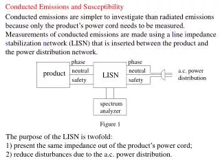
Principle of operation of switching dc power supplySwitching Freq = 1/T = 20 kHz – 500 kHzDuty cycle “τ/T” regulates (adjusts) output dc voltage level VL Lecture 12 Radiated Emissions
Use of common mode choke and capacitive filtering between ac power line and an electronic device to reduce both conducted common-mode and differential mode conducted RF emissions Black The “green wire” RF choke Lgw discourages common-mode RF currents on the Phase and Neutral wires from returning to the metal chassis of the product via the green (3rd prong) wire. White Green LISN – Line isolation stabilization network (May be replaced by ac power cord.) “3rd Prong” Lecture 12 Radiated Emissions