Perpendicular transport/diffusion
Turbulence, magnetic field complexity and perpendicular transport of energetic particles in the heliosphere W H Matthaeus Bartol Research Institute, University of Delaware Collaborators: G. Qin, J. Bieber, D. Ruffolo, P. Chuychai. Perpendicular transport/diffusion.

Perpendicular transport/diffusion
E N D
Presentation Transcript
Turbulence, magnetic field complexity and perpendicular transport of energetic particles in the heliosphereW H MatthaeusBartol Research Institute, University of DelawareCollaborators: G. Qin, J. Bieber, D. Ruffolo, P. Chuychai
Perpendicular transport/diffusion • Field Line Random Walk (FLRW) limit is a standard picture. • K (v/2) D Fokker Planck coefficient for field line diffusion
“BAM” theory of perp diffusion Bieber and Matthaeus, 1997 TGK formula for diffusion Ansatz #1: form of v-v correlation Ansatz #2: effective collision time BAM result
Puzzling properties of perpendicular transport/diffusion Computed K’s fall Well below FLRW at low energy, but above hard sphere and BAM theories • Numerical results support FLRW at high energy, but no explanation for reported low energy behavior • K may be involved in explaining observational puzzles as well • Enhanced access to high latitudes • “chanelling” Slab/2D and Isotropic (Giacalone And Jokipii.) Slab (Mace et al, 2000) FLRW BAM
Importance of turbulence geometry and structure • In parallel scattering, the distribution of turbulence energy over wave vector direction, as well as the wave vector magnitude, is very important. • In perpendicular scattering, the spectral characteristics are also important, especially the transverse complexity and structure of the magnetic field. Bieber et al, 1994. Schlickesier et al, 1994, Droege 2002
Correlation/Spectral anisotropy MHD Anisotropy: dynamical development oftransverse complexity
Shredding of flux tubes in 3D Two component Model is three-dimensional: 20% slab + 80% 2D 1D slab only
Subdiffusive regime Slab or near-slab models: very little transverse complexity
Numerical Results: 0.9999 slab fluctuations:Parallel and perpendicular transport in the same simulation! • Running diffusion coefficient: K = (1/2) d<2>/dt • Parallel: free-streaming, then diffusion ( QLT) • Perpendicular: initially approaches FLRW, but is thwarted…behaves as t-1/2 i.e., subdiffusion Qin et al, 2002
IH Urch, Astrophys. Space Sci., 46, 389 (1977). J. Kota and J.R. Jokipii Ap. J. 531, 1067 (2000) Perpendicular Subdiffusion • In evaluating K~z/t Dinstead of using z/t =v, assume that the parallel motion is diffusive, and z =(2 K t )1/2 • K = D (K / t)1/2 • For this to occur, nearby field lines must be correlated. If the transverse structure sampled by the particle becomes significant, can diffusion be restored?
Recovery of diffusion Turbulence with adequate transverse complexity
Numerical simulation using 2-component turbulence:80% 2D + 20% slab Qin et al, 2002 Running diffusion coefficients vs. time • Parallel: free stream, then diffuse, but at level < QLT • nonlinear effect of 2D fluctuations • Perpendicular: evolves towards FLRW, subsequent decrease, and then a regime of “second diffusion” emerges.
Perpendicular diffusion: Loss and recovery • Subdiffusion (Urch-type) should be taken seriously • Subdiffusion always occurs in slab geometry • FLRW rarely if ever works (but may be the “target”) • BAM theory doesn’t work either • Composite geometry simulations provide insight: • FLRW and BAM tend to bracket computed results • Kperp/Kpar ~ constant as function of rigidity (0.02-0.05) in some parameter regimes • Numerical evidence points to need for a nonlinear theory • FLRW + parallel scattering not enough • Require an additional source of randomization Interaction between transverse complexity of the field and particle gyro-orbits
How much transverse structure is sampled by particles ? slab • Slab field lines are identical • No field line separation • 2D field lines are trapped on flux surfaces • ”escape” catalyzed by slab component • Most effective separation when: • Field is 3D (e.g., slab+2D mixture) • Gyro-orbits sample transverse structure 2D 2D+slab 50-50 See Ruffolo and Matthaeus, in preparation, 2002
Recovery by stochastic instability Rechester and Rosenbluth PRL, 1978 • Field lines exponentially separate • Field line mapping is reversible diffusion is destroyed • Add scattering restore diffusion • Weak collisions destroy reversibility and restore FLRW • Stronger scattering balance between stretching and scattering • Chandran and Cowley (PRL, 1998) modify R+R for collisonless case See also Kadomtsev and Pogutse, 1979
A new theory of nonlinear perpendicular (guiding center) diffusion • Begin with Taylor Green Kubo formula for diffusion • Key assumption: perpendicular diffusion is controlled by the motion of the particle guiding centers. Replace the single particle orbit velocity in TGK by the effective velocity • TGK becomes
Nonlinear perpendicular diffusion (1) • Simplify 4th order to 2nd order (ignore v-b correlations: e.g., for isotropic distribution…) • Special case: parallel velocity is constant and a=1, recover QLT/FLRW perpendicular diffusion. (Jokipii, 1966) Model parallel velocity correlation in a simple way:
Nonlinear perpendicular diffusion (2) • Corrsin independence approximation The perpendicular diffusion coefficient becomes Or, in terms of the spectral tensor
Nonlinear perpendicular diffusion (3) • “Characteristic function” – here assume Gaussian, diffusion probability distribution After this elementary integral, we arrive at a fairly general implicit equation for the perpendicular diffusion coefficient
Nonlinear perpendicular diffusion (4) • The perpendicular diffusion coefficient is determined by • To compute Kxx numerically we adopt particular 2-component, 2D - slab spectra • These solutions are compared with direct determination of Kxx from a large number of numerically computed particle trajectories in realizations of random magnetic field models. We find very good agreement for a wide range of parameters. and solve
Comparison of Nonlinear theory with simulations • Low dB/B= 0.2 • Parallel scattering nearly QLT • NL GC theory accounts well for perpendicular transport
Comparison for strong turbulence: Four theories • db/B = 1 • FLRW never very good • BAM good at large rL/Lc • RR-CC good at low rL/Lc • NLGC theory remains accurate for wide range of rL/Lc
Parallel vs. Perpendicular diffusion • Not a purely linear relationship • Kperp << Kpar
G. Qin et al, 2002 GRL G. Qin et al 2002 ApJL Matthaeus et al, 2002 Perpendicular transport • Particle gyrocenters try to follow fields lines (“FLRW” limit) • Motion along field lines is inhibited by parallel (pitch angle) scattering • Low transverse complexity subdiffusion • Strong transverse complexity recovery of diffusion at lower level than FLRW • A nonlinear theory of guiding center diffusion agrees well with simulations • Comparisons with observations are underway
Some remaining problems in perpendicular transport • Observational connections • Transition between subdiffusion and diffusion • Channeling and sharp boundaries (conditional/inhomogeneous statistics) • Dynamical effects (random dynamical effects can be incorporated easily in the present formalism!) • Inhomogenous large scale field, e.g., Fisk field • Field line separation effects (in progress, with D. Ruffolo) • Anisotropic FLRW (ICRC proceedings, Ruffolo, Chuychai and Matthaeus
K┴ / K║= const (as a function of rigidity)in some parameter regimes • Results of Giacalone & Jokipii (left) as well as Qin (right) indicate K┴ / K║ ~ 0.02-0.04 at typical cosmic ray energies
K┴Determined from Jovian Electrons From Chenette et al., Astrophys. J. Lett., L95-L99, 1977. Concept: Jupiter is a near “point source” of electrons. Longitudinal spread of electrons at 1 AU provides a direct measure of K┴ Curve a: K┴ = 5X1020 cm2/s Curve b: K┴ = 1021 cm2/s Summary of Results for ~2 MV Jovian electrons: K┴ = 7 x 1020 cm2/s; λ┴ = 0.0047 AU K║ = 5 x 1022 cm2/s; λ║ = 0.33 AU K┴ / K║ = 0.014
Comparison for strong turbulence • Db/B = 1 • Parallel scattering differs from QLT • NL GC theory remains accurate for wide range of rL/Lc
Slab Geometry: Wavevectors k parallel to mean field B0. Fluctuating field δB perpendicular to B0. Motivations: Parallel propagating Alfvén waves. Computational simplicity. 2D Geometry: k and δB both perpendicular to B0. Motivations: “Structures.” Turbulence theory. Laboratory experiments. Turbulence Geometry
Spectral method simulations: cross sections of magnetic energy density B0 X,z cross sections Transverse Section x,y Dmitruk and Matthaeus, 2002
SW turbulence “sees” at least two preferred directions: radial (expansion) local mean magnetic field Several observational studies confirm lack of isotropy Multicomponent models: each with fixed symmetry Two/Three component “slab” + quasi-2D + “structures” model seems to cover most of the constraints: scattering theory direct observations “Maltese cross” Weakly Compressible MHD theory Slab component: waves/origin of SW quasi-2D component: consistent with simulations, theory and lab experiments. Structures: smaller parallel variance piece (phase mixing, compressible simulations, “5:4:1”, NI Theory) Symmetry/Anisotropy has major impact on transport, heating, couplings to kinetic effects, diffusion, etc... Anisotropy and symmetry Maltese Cross Simulations and Theory suggest that perpendicular cascade is much faster than parallel
Recovery by stochastic instability Rechester and Rosenbluth PRL, 1978 • Field line distribution is an area preserving map • Field line complexity grows as field lines exponentially separate • Map is reversible diffusion is destroyed • Add perpendicular displacements due to scattering restore diffusion • A small amount of collisional scattering destroys reversibility and restores to QLT/FLRW value • Stronger scattering balance between stretching and scattering Scale for decorrelation of random displacements
Rechester and Rosenbluth (1978) form: Decorrelation determined by exponential separation of field lines Chandran and Cowley (PRL, 1998) Modify R+R for collisonless case: The RR-CC nonlinear perpendicular Diffusion coefficient becomes: