Download
1 / 20
200 likes | 217 Views
More Searching. Dan Barrish-Flood. Running time of Dynamic Set Operations. we’ve seen that all our dynamic set operations can be done in Θ( h ) time (worst-case) on a binary search tree of height h. a binary search tree of n nodes has height Θ(lg n )

E N D
More Searching Dan Barrish-Flood 4a-Searching-More
Running time of Dynamic Set Operations • we’ve seen that all our dynamic set operations can be done in Θ(h) time (worst-case) on a binary search tree of height h. • a binary search tree of n nodes has height Θ(lgn) • so all dynamic set operations take Θ(lgn) time on a binary search tree. • right? WRONG! • insert these numbers to form a binary search tree, in this order: 1, 2, 3, 4, 5 4a-Searching-More
Binary Search Tree Random Insertion & Deletion • What is the average depth of a BST after n insertions of random values? • The root is equally likely to be the smallest, 2nd smallest, ..., largest, of the n values. So with equal probability, the two subtrees are of sizes 1 & n-2 (not n-1, don’t forget the root!) 2 & n-3 ... n-3 & 2 n-2 & 1 Wait til you see the next slide!... 4a-Searching-More
Random Insertion/Deletion (Cont’d) • The analysis is identical to Quicksort! • The root key is like the pivot. • So n insertions take O(nlgn) on average, thus each insertion takes O(lgn), which is the tree height. 4a-Searching-More
Balanced Search Trees • Careful, I may have used BST in the past for “binary search tree” not “balanced search tree”, I will try to avoid this confusion! • The general idea (there are exceptions) • do extra work during INSERT and DELETE to ensure the tree’s height is Θ(lgn) • the rest of the dynamic set operations are unchanged. • Two examples: • Red-Black Trees (CLRS ch. 13) • elegant definition • wicked hairy insert/delete • 2-3 Trees • simpler to understand • not true binary trees 4a-Searching-More
a taste of Red-Black Trees • a Red-Black tree is a binary search tree where • the root is BLACK • each node is colored RED or BLACK • every leaf is black • each of a red node’s children are black • every path from a node to one of its descendant leaves contains the same number of black nodes • (a minor twist: we consider the NIL’s as leaves, and all the nodes with keys as internal nodes) • the height of a node (for trees in general) is the # of edges on the longest downward path from that node to a leaf. 4a-Searching-More
RBT, each leaf (NIL) is black the tiny number next to a node is its “black-height” 4a-Searching-More
Dynamic Set Operations as implemented with RBT’s It’s not that hard to prove (by induction) that the RBT properties imply: • a RBT with n internal nodes has height ≤ 2 lg(n+1) • don’t worry about the proof, but see CLRS p. 274 if you’re interested in the details • The height of a RBT is O(lgn), so all dynamic set operations run in O(lgn) time. • But wait! INSERT, DELETE may destroy the RBT property! But, it turns out, these two operations can indeed be supported in O(lgn) time, too. 4a-Searching-More
More on tree-traversal, here is pre-order traversal (note this is not a binary tree) First “process” (e.g. print) the root (hence pre), then recursively process the root’s left subtree(s), then recursively process the root’s right subtree(s). For this tree, we get 1,2,3,...,9 4a-Searching-More
More on tree traversal, here is post-order traversal (note this is not a binary tree) First recursively process the root’s left subtree(s), then recursively process the root’s right subtree(s), then lastly (hence post) “process” (e.g. print) the root. For this tree, we again get 1,2,3,...,9 4a-Searching-More
2-3 Trees • Another kind of Balanced Search Tree • What are the structural requirements: • every non-leaf (i.e. internal) node has exactly 2 or 3 children • all leaves are at the same level • here are three 2-3 trees (not showing keys!) 4a-Searching-More
2-3 Trees, more structural info • the “thinnest” 2-3 tree is a complete binary tree (see picture on prev. slide) • the “fattest” 2-3 tree is a complete 3-ary tree (again see prev. slide). • If the tree has height h, (recall all leaves are at the same level), the number of leaves, l, is between 2h and 3h. • A 2-3 tree of n nodes (total) has a height between log3n and log2n, and since log3n = log32 x log2n (why?), the height h is guaranteed to be within a small constant factor of log2n. 4a-Searching-More
Where is the data in a 2-3 tree? All the records (keys, other satellite data) are in the leaves. The records are in sorted order. Each internal node has one or two guides: the greatest value in its leftmost one (or two) subtree(s). 4a-Searching-More
Searching in a 2-3 Tree: Suppose I’m searching the above 2-3 tree (the one with the guides 8, 29 in the root) for the key 27. Start at the root. 27 ≤ 8? No, so forget about the root’s leftmost subtree. 27 ≤ 29? Yes, so we know our target (if it exists) is in the root’s middle subtree. Thus proceed to the node directly below the root? 27 ≤ 11? No. So forget about this node’s leftmost subtree. 27 ≤ 21? No, so we know our target (if it exists) must be in this node’s rightmost subtree. So follow our current node’s rightmost pointer down. We’re at a leaf (the good stuff is in here!), and we find our target 27 stored in this leaf. We use this method to always reach the “right” leaf, where we will either find our target in that leaf, or find that our target does not exist. SEARCH(2-3_tree, key) clearly, because of the height of the tree, runs in worst-case time O(lg n). I don’t have any good pseudo-code (maybe I’ll make or find some) for this routine. 4a-Searching-More
2-3 Tree Insert (let’s insert 15 into the prev. tree) tree has increased in height! 4a-Searching-More
2-3 Tree Delete; let’s delete 10 from the 1st tree to get the 2nd one (one method). here we stole 11 from a sibling 4a-Searching-More
2-3 Tree Delete; let’s delete 10 from the 1st tree to get the 2nd one (other method). here we merged nodes 4a-Searching-More
2-3 Tree Delete; let’s delete 3 from the 1st tree to get the 3rd, there’s just one way). again, we stole from a sibling 4a-Searching-More
2-3 Tree Delete; let’s delete 5 tree loses a level! 4a-Searching-More