Download
1 / 16
160 likes | 294 Views
Reconstruction PDF in Inhomogeneous Ice. Ribordy & Japaridze Université de Mons-Hainaut AMANDA/ICECUBE Berkeley – March '05. conv. Pandel patch pandel conv. Pandel, optimized parameters. patch Pandel reconstructed track. true track. min. bias corsika sample

E N D
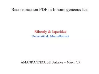
Reconstruction PDF in Inhomogeneous Ice Ribordy & Japaridze Université de Mons-Hainaut AMANDA/ICECUBE Berkeley – March '05
conv. Pandel patch pandel conv. Pandel, optimized parameters patch Pandel reconstructed track true track min. bias corsika sample patch Pandel distribution is compared to the reconstructed and MC time residual distribution Introduction 1. patch Pandel conv. Pandel: we want to use conv. Pandel, because one gets rid of time residual peak artefacts 2. The phenomenological parameters should be adjusted because at short distances, conv. Pandel is peaking at slightly different time residuals compared to patch Pandel if we use the same (lambda, tau)
Introduction But after the adjustment of parameters in the convoluted Pandel, only modest improvements in reconstruction results (see talk AMANDA@Bommerholz, June 04) go beyond this approach and explore new paths, given Pandel assumes an isotropic point –like emitter. Therefore, it does not describe the time residual distributions for 1) the anisotropic Cerenkov emission 2) along a (infinite, minimum ionizing muon) track 3) in a medium with non-constant optical properties. AMANDA ice: the characteristic lengths vary considerably w.r.t. the depth a) We consider the depth-dependence of the ice parameters fit (tau,lambda) locally (and not globally as in Bommerholz) b) We provide a prescription on the accounting of variable ice properties in the Pandel parameters for reconstruction see AMANDA Internal Report 20050301 Ribordy/Japaridze, "Reconstruction PDF in an Inhomogeneous Medium" TODAY
Introduction Pandel PDF (including absorption): is a solution to: drawing from Pandel thesis
TWR exp. data: constant tau MC data: smooth increase of tau, vary significantly tau-lambda behavior (Bommerholz, June 04) • lambda: looks ¨compatible¨ • vary significantly with distance MC VS exp. : not exactly the same behavior. What do we do ?
from http://amanda.berkeley.edu/kurt/ice2000 Ice parameters VS Pandel • ice properties drastically change w.r.t. the depth • a change in the effective scattering length • affects the distribution relatively more than a • change in the absorption length • (we assume here that l = les(valid for this consideration as we will see))
we write where 2-layer PDF derivation we define the 2-layer PDF: • where layer i has optical properties (ri,li). • the model is rudimentary: spherical symmetry is broken into cylindrical: • valid at big distances • valid at short distance (length scale of variation of the optical parameters is longer than the distance scale)
2-layer PDF analytical closed form exact solution:
where l = labs or les N-layer generalisation 2 N layer: if ri = rj = r, then we can solve the product analytically: where This result in the general case where l and r vary simultaneously could not be formally demonstrated. Conclusion: varying l and r separately (with r changing slowly), we have the averaging formulas:
N-layer PDF convoluted with time jitter: from AMANDA Internal Report 20031201, Japaridze/Ribordy, "Photon Arrival Time Distribution Convoluted to a Gaussian Time Measurement Uncertainty" We have then a clear prescription to account for variable ice properties in reconstruction (within the validity of the model). This model allowed to demonstrate this simple prescription
MC time residual distribution • We want now to show that ice properties really impact on the time residual distributions • We choose MC in control of the input ice model, knowledge of the physical events (with exp. data, we would have to rely on the reconstruction results). • However, MC is based on PTD the ice properties are the ones prevailing at the receiver ("local bulk ice") • sample of dcorsika MC • extract "unbiased" time residual distributions from MC: - a (1) single(2) crossing muon - (3) good(4) optically readout OM with (5) exactly 1 hit, within some (6) TOT range good statistics on a wide range of depths and distances time residual distr. assumed to match the single PE distribution (mean unbiased)
MC time residual distribution -285m -245m -205m -165m -125m -85m -45m -5m +35m +75m +115m +155m +195m +235m +275m +315m
MC time residual distribution • projection for each distance, for each depth • fit (t , l) with p, fixed distance and labs lambda range corresponds almost to the les range tau seems to be correlated as well to les. Consider tau constant w.r.t. the depth (but function of distance) 30 m 60 m
MC time residual distribution MC time residual distribution fit:
About reconstruction • to speed conv. Pandel (~3 times slower than patch Pandel) • table recover patch Pandel speed • variable ice : • "local bulk ice" as fast as conv. Pandel • "photonics ice" (using the prescription) • about 2 times slower than conv. Pandel • single PDF table: not possible with variable ice due to lack of • scaling properties of the PDF
Conclusion • necessary to account for ice properties in reconstruction (and not only in MC) • clear averaging prescriptions were presented (though not demonstrated when both lambda's simultaneously vary. • table PDF: unfortunately, no adequate scaling of p was found when both lambda's simultaneously vary, so that it should be slower by factor ~5, using the prescription (local bulk ice reconstruction ~ 3 times slower) • further studies: reconstruction performance should be investigated • photonics in future: a nice tool to check the prescription • go beyond point-like isotropic emitter picture (extend the prescription to the track picture) • implementation influences software design


![[PDF] Free Download The Girl in the Ice By Robert Bryndza](https://cdn4.slideserve.com/8331744/slide1-dt.jpg)