CAS 2017 Vacuum simulations
110 likes | 130 Views
Learn how to set up geometric elements in Molflow for vacuum simulations on coated samples. Practice pressure calculations, gas injection rates, and transmission ratios.

CAS 2017 Vacuum simulations
E N D
Presentation Transcript
CAS 2017Vacuum simulations Individual work - exercises
Gauge 2 Gauge 1 Coated sample
Gauge 2 Gauge 1 1000 mm ~250 mm 63 mm Coated sample ~150 mm ~150 mm
Setting up the geometry in Molflow 1000 mm 63 mm Coated sample • Create the base tube with the Test / Pipe command • Use the (distorted) Scale command to get dimensions right
Setting up the geometry in Molflow Coated sample ~150 mm ~150 mm • Use the Extrude command to create two more sections
~250 mm Coated sample • Use the Rotate facet and Move facet commands with the copy option to create the perpendicular tubes • Then use the build intersection command to create the union of the two pipes (select intersecting facets, and select all vertices that you’d like to keep) • The build intersection command works correctly if one pipe is slightly thicker than the other (use Scale facet)
Formula for pressure on facet N: “PN” Gauge 2 Gauge 1 Coated sample • Use the end caps of the tubes to represent the gauges (use formulas), pumps (use sticking) and gas injection Q S = 300 l/s
Gauge 2 Gauge 1 Coated sample • Recommended: create a transparent facet that runs along the centerplane, and add profile and texture to it
Exercise 1 • We start inject gas at a constant rate. After some time the pressures stabilize. We observe the following pressures on the gauges: • Gauge1: 1E-6 mbar • Gauge2: 2.5E-9 mbar • Approximately what’s the sticking factor of the sample? • What’s the gas injection rate? 2.5E-9 mbar 1E-6 mbar Sticking = ? Coated sample Q=?
Exercise 2 • NEG coating is an effective pump, but it can’t pump gas forever: eventually it saturates. Its pumping ability drops quickly when the pumped gas forms one monolayer on the surface – corresponding to about 1E15 pumped molecules / cm2 • In our setup, how much N2 is that? • How much time does it take until our setup saturates?
Exercise 3 • In the first exercise you have found the sticking factor for a given pressure ratio, observed on the two gauges. • What was the transmission ratio of the gas (the probability that an injected molecule makes it through the tube) for that pressure ratio? • By changing the simulation parameters, you could help an engineer to solve exercise 1 in the future. Make a “transmission ratio as a function of the sample’s sticking factor” plot: • X axis: different sticking factor values (around 5-7 different values) • Y axis: gas transmission ratio