Download
1 / 32
330 likes | 529 Views
SURFACE WAVE SURVEYS LIMITED. Non-intrusive measurement of ground stiffness. Website: www.surfacewavesurveys.co.uk E-mail: info@surfacewavesurveys.co.uk. Idealised stiffness - strain behaviour exhibited by most soils. The CSWS measures Gmax.

E N D
SURFACE WAVE SURVEYS LIMITED Non-intrusive measurement of ground stiffness Website: www.surfacewavesurveys.co.uk E-mail: info@surfacewavesurveys.co.uk
Idealised stiffness - strain behaviour exhibited by most soils The CSWS measures Gmax. Gop/Gmax is 0.5 to 0.8 for soils and near unity for sands and soft rocks. Stiffness values can be converted to Young’s Modulus (E) using Poisson’s ratio () E = 2(1+ )G
The different types of seismic wave Energy source Geophone detector Ground level Surface waves Shallow reflection Boundary between earth layers Refraction Deep reflection Body waves: reflections and refractions Two types: P-waves (Pressure waves) S-waves (Shear waves) Surface waves Two types: Love waves (A type of S-wave) Rayleigh waves (Neither P- nor S- waves)
Seismic wave particle motion Direction of propagation P- Wave Direction of movement S-Wave Direction of propagation Direction of movement (Or any other direction at right angles to the propagation direction) Rayleigh Wave Direction of propagation Direction of movement
The surface wave method Frequency controlled vibrator 2Hz natural frequency geophones Amplifier unit Controller unit
CSWS principle of operation (1) • A range of frequencies is selected and the vibrator, under computer control, automatically shakes the ground at each frequency throughout this range. • For each frequency the surface waves are detected by the geophones which send signals representing the ground motion as a function of time back to the controller. • This data is Fourier transformed to give the phase of the Rayleigh wave at each geophone position.
CSWS principle of operation (2) • The gradient of the phase-distance relationship gives the wavelength of the Rayleigh wave. • The wavelength and frequency of the Rayleigh wave give its velocity. • Elastic theory is used to convert the Rayleigh wave velocity to the shear wave velocity and the shear wave velocity to the stiffness. • The stiffness value is allocated to a depth which is 1/3 of the Rayleigh wave wavelength (/3 inversion).
Calculation of Rayleigh wave velocity Frequency = f Distance between geophones = d Phase difference = 2 -1 = By proportion = d 360 Therefore = 360.d And Rayleigh wave velocity V = f d R 1 2 By knowing the frequency, f, and the change in phase with distance from the vibrator, d, we can determine the Rayleigh wave velocity, V . R
Calculation of stiffness From the theory of elasticity VS = Shear wave velocity VR = Rayleigh wave velocity P = f(Poisson’s ratio ) for = 0.25, P = 1.09 for = 0.50, P = 1.05 G = Shear modulus = Bulk density VS = PVR G = VS2 = P2VR2
Depth (m) Chalk under shallow fill 0 1000 2000 3000 4000 5000 0 Fill -5 Dense chalk -10 -15 -20 -25 -30 Gmax (MPa)
Stiffness inversion due to buried alluvium 0 50 100 150 200 250 300 Fill 0 Soft, grey, slightly sandy silty clay [Alluvium] Depth (m) Medium dense, sub-angular to sub-rounded sandy fine to medium flint gravel -5 -10 -15 Gmax (Mpa)
Depth (m) Gmax (Mpa) Sequence of clays 0 200 400 600 800 0 Weathered, sandy clay -5 Silty clay -10 -15 Clay marl -20 -25 -30 -35
Example of using CSWS to measure the degree of ground improvement resulting from the insertion of vibro stone columns 0 20 40 60 80 100 120 140 160 180 0 -2.00 -4.00 Depth (m) -6.00 -8.00 -10.00 -12.00 -14.00 Gmax (Mpa) Column diameter 500mm Depth 6m Triangular grid spacing 1500mm By courtesy of Keller Ground Engineering
Dynamic compaction with 1.75m stone pillars From Moxhay et al. (2001)
Vibro stone columns with surface tamping – deep ash fill From Moxhay et al. (2008)
Stiffness increase after a temporary loss during ground treatment
Settlement prediction from CSW data Required information: CSW stiffness/depth profile, foundation shape, size, depth below ground and load. • The sub-surface is divided into layers and average Gmax values are found for each. • The initial value of Young’s Modulus E for each layer is taken to be 2.5Gmax (average). • The vertical stress at the centre of each layer is found using the appropriate Boussinesq formula. • Initial values of strain for each layer are found from the vertical stress and initial E values. • These strains will be too high to relate to the CSW Gmax values. The E values are therefore revised using factors from a standard curve of stiffness against strain (see Moxhay at al. (2008) Appendix 2). • The calculations are repeated to produce new strains. • After repeating several times the new E values converge to the previous ones. • The settlement in each layer is calculated by multiplying the final strain by the layer thickness. • Addition of the settlements in each layer gives the total settlement.
Vibro stone column site - example data for settlement calculation From Moxhay et al. (2008)
Example settlement calculation • Originally calculated settlement: 60mm. • Settlements for whole site calculated from CSW data varied between 6mm and 15mm, average: 11mm. • Observed settlement after four years: 10mm.
Example of the effect on CSWS results of a very hard raft of material near the surface
Advanced processing of CSW data using WinSASW2 software with PreCSW • An experimental dispersion curve for input to WinSASW2 is prepared from the field data using PreCSW. • A polynomial, called the representative dispersion curve, is fitted to it. This essentially produces a smoothed version of the field data. • An initial estimate of the earth model in terms of layer thicknesses is made. • The dispersion curve that would be produced by this model is generated and superimposed on the smoothed experimental one. • Adjustments to the model are made to produce a reasonable fit. • The best-fit model is used as the starting point for the main matrix inversion. Initially, layer thicknesses are held constant and the optimum velocities found by iteration. • Thickness and velocity are then iterated together to produce the final result.
Example WinSASW2 output - a steady increase of stiffness with depth By courtesy of ESG Pelorus Surveys
Example WinSASW2 output – a stiffness inversion By courtesy of ESG Pelorus Surveys
Example WinSASW2 quality control (1) Criteria for a satisfactory result: • The model is plausible. • The dispersion curve for the model and the representative dispersion curve are a good match. • The resolution of the shear wave velocity does not fall below 0.1.
Example WinSASW2 quality control (2) Index for the different dispersion curves:Grey - ExperimentalBlue - RepresentativeRed - Final model By courtesy of ESG Pelorus Surveys
Advantages of the CSWS • Non – invasive. • Representative. • Independent of soil type. • Quick. • Portable. • Low – cost. • Provides a direct route to settlement prediction.
Future development • Processing software enhancement. The Unbiased Short Array (USA) Beamforming Technique, currently under development by Professor Joh in South Korea, will improve the results produced by WinSASW2.