Download
1 / 80
800 likes | 971 Views
Feature Detection and Matching. Reading: Szeliski Chapter 4 Pages: 208~266. http://staff.ustc.edu.cn/~xjchen99/teaching/teaching.html. Image Matching. by Diva Sian. by swashford. TexPoint fonts used in EMF. Read the TexPoint manual before you delete this box.: A A A A A A.

E N D
Feature Detection and Matching Reading: Szeliski Chapter 4 Pages: 208~266 http://staff.ustc.edu.cn/~xjchen99/teaching/teaching.html
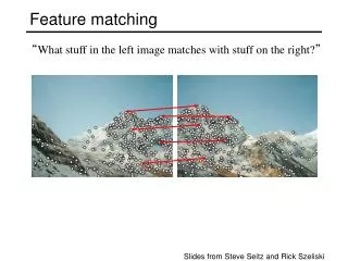
Image Matching by Diva Sian by swashford TexPoint fonts used in EMF. Read the TexPoint manual before you delete this box.: AAAAAA
Harder Case by Diva Sian by scgbt
Even Harder Case “How the Afghan Girl was Identified by Her Iris Patterns” Read the story
Harder still? NASA Mars Rover images
Answer below (look for tiny colored squares…) NASA Mars Rover images with SIFT feature matchesFigure by Noah Snavely
Features All is Vanity, by C. Allan Gilbert, 1873-1929 • Readings • Szeliski, Ch 4.1 • (optional) K. Mikolajczyk, C. Schmid, A performance evaluation of local descriptors. In PAMI 27(10):1615-1630 • http://www.robots.ox.ac.uk/~vgg/research/affine/det_eval_files/mikolajczyk_
Invariant Local Features Find features that are invariant to transformations • geometric invariance: translation, rotation, scale • photometric invariance: brightness, exposure, … Feature Descriptors
Advantages of Local Features Locality • features are local, so robust to occlusion and clutter Distinctiveness: • can differentiate a large database of objects Quantity • hundreds or thousands in a single image Efficiency • real-time performance achievable Generality • exploit different types of features in different situations
More Motivation… Feature points are used for: • Image alignment (e.g., mosaics) • 3D reconstruction • Motion tracking • Object recognition • Indexing and database retrieval • Robot navigation • … other
Features • Point/patch, • Edge/curve • Region
Want Uniqueness • Look for image regions that are unusual • Lead to unambiguous matches in other images • How to define “unusual”?
Corner Detection • Basic idea: Find points where two edges meet—i.e., high gradient in two directions • “Cornerness” is undefined at a single pixel, because there’s only one gradient per point • Look at the gradient behavior over a small window • Categories image windows based on gradient statistics • Constant: Little or no brightness change • Edge: Strong brightness change in single direction • Flow: Parallel stripes • Corner/spot: Strong brightness changes in orthogonal directions
Matching Criterion • (weighted) Summed Square Difference – SSD • Compare an image patch against itself
Local Measures of Uniqueness Suppose we only consider a small window of pixels • What defines whether a feature is a good or bad candidate? Slide adapted from Darya Frolova, Denis Simakov, Weizmann Institute.
Feature Detection Local measure of feature uniqueness • How does the window change when you shift it? • Shifting the window in any direction causes a big change “corner”:significant change in all directions “flat” region:no change in all directions “edge”: no change along the edge direction Slide adapted from Darya Frolova, Denis Simakov, Weizmann Institute.
Feature Detection: Mathematics • Consider shifting the window W by (u,v) • how do the pixels in W change? • compare each pixel before and after bysumming up the squared differences (SSD) • this defines an SSD “error” of E(u,v): W
Auto-correlation function Window function Shifted intensity Intensity Window function w(x,y) = or 1 in window, 0 outside Gaussian Harris Detector: Mathematics Change of intensity for the shift [u,v]:
Auto-Correlation Function Good unique minimum 1D aperture problem No good peak
Small Motion Assumption • Taylor Series expansion of I: • If the motion (u,v) is small, then first order approx is good
Feature Detection: Mathematics • Image gradient • Harris detector with a [-2,-1,0,1,2] filter for Ix • Gaussian filter
Small Motion Assumption • Plugging this into the formula on
Feature Detection: Mathematics This can be rewritten: Auto-correlation matrix x- x+
Feature Detection: Mathematics • For the example above • You can move the center of the blue window to anywhere on the blue unit circle • Which directions will result in the largest and smallest E values? • We can find these directions by looking at the eigenvectors ofH
Quick eigenvalue/eigenvector review The eigenvectors of a matrix A are the vectors x that satisfy: The scalar is the eigenvalue corresponding to x • The eigenvalues are found by solving: • In our case, A = H is a 2x2 matrix, so we have • The solution: Once you know , you find x by solving
Feature Detection: Mathematics This can be rewritten: x- x+ • Eigenvalues and eigenvectors of H • Define shifts with the smallest and largest change (E value) • x+ = direction of largest increase in E. • + = amount of increase in direction x+ • x- = direction of smallest increase in E. • - = amount of increase in direction x+
Feature Detection: Mathematics Intensity change in shifting window: eigenvalue analysis 1, 2 – eigenvalues of H If we try every possible orientation n, the max. change in intensity is 2 Ellipse E(u,v) = const (max)-1/2 (min)-1/2
Feature Detection: Mathematics 2 Classification of image points using eigenvalues of M: “Edge” 2 >> 1 “Corner”1 and 2 are large,1 ~ 2;E increases in all directions 1 and 2 are small;E is almost constant in all directions “Edge” 1 >> 2 “Flat” region 1
Feature Detection: Mathematics • How are +, x+, -,and x+ relevant for feature detection? • What’s our feature scoring function?
Feature Detection: Mathematics • How are +, x+, -,and x+ relevant for feature detection? • What’s our feature scoring function? • Want E(u,v) to be large for small shifts in all directions • the minimum of E(u,v) should be large, over all unit vectors [u v] • this minimum is given by the smaller eigenvalue (-) of H
Feature Detection • Here’s what you do • Compute the gradient at each point in the image • Create the H matrix from the entries in the gradient • Compute the eigenvalues. • Find points with large response (-> threshold) • Choose those points where - is a local maximum as features
Feature Detection • Here’s what you do • Compute the gradient at each point in the image • Create the H matrix from the entries in the gradient • Compute the eigenvalues. • Find points with large response (-> threshold) • Choose those points where - is a local maximum as features [Shi and Tomasi 1994]
Harris Detector Harris and Stephens 1988 Measure of corner response: (k – empirical constant, k = 0.04-0.06) • The trace is the sum of the diagonals, i.e., trace(H) = h11 + h22 • Very similar to - but less expensive (no square root)
Harris Detector: Mathematics 2 “Edge” “Corner” • R depends only on eigenvalues of H • R is large for a corner • R is negative with large magnitude for an edge • |R| is small for a flat region R < 0 R > 0 “Flat” “Edge” |R| small R < 0 1
Harris Detector • The Algorithm: • Find points with large corner response function R (R > threshold) • Take the points of local maxima of R
Harmonic Mean Brown, M., Szeliski, R., and Winder, S. (2005). • Smoother function in the region where
Harris Detector: Workflow Compute corner response R
Harris Detector: Workflow Find points with large corner response: R>threshold
Harris Detector: Workflow Take only the points of local maxima of R
Example: Gradient Covariances Corners are whereboth eigenvalues are big from Forsyth & Ponce Detail of image with gradient covar- iance ellipses for 3 x 3 windows Full image
Example: Corner Detection (for camera calibration) courtesy of B. Wilburn
Example: Corner Detection courtesy of S. Smith SUSAN corners