Lecture 9

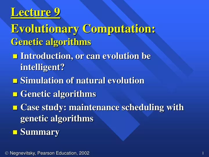
1. Lecture 9 Evolutionary Computation: Genetic algorithms • Introduction, or can evolution be intelligent? • Simulation of natural evolution • Genetic algorithms • Case study: maintenance scheduling with genetic algorithms • Summary

2. Can evolution be intelligent? • Intelligence can be defined as the capability of a system to adapt its behaviour to ever-changing environment. According to Alan Turing, the form or appearance of a system is irrelevant to its intelligence. • Evolutionary computation simulates evolution on a computer. The result of such a simulation is a series of optimisation algorithms, usually based on a simple set of rules. Optimisation iteratively improves the quality of solutions until an optimal, or at least feasible, solution is found.

3. The behaviour of an individual organism is an inductive inference about some yet unknown aspects of its environment. If, over successive generations, the organism survives, we can say that this organism is capable of learning to predict changes in its environment. • The evolutionary approach is based on computational models of natural selection and genetics. We call them evolutionary computation, an umbrella term that combines genetic algorithms,evolution strategiesandgenetic programming.

4. Simulation of natural evolution • On 1 July 1858, Charles Darwin presented his theory of evolution before the Linnean Society of London. This day marks the beginning of a revolution in biology. • Darwin’s classical theory of evolution, together with Weismann’s theory of natural selection and Mendel’s concept of genetics, now represent the neo-Darwinian paradigm.

5. Neo-Darwinism is based on processes of reproduction, mutation, competition and selection. The power to reproduce appears to be an essential property of life. The power to mutate is also guaranteed in any living organism that reproduces itself in a continuously changing environment. Processes of competition and selection normally take place in the natural world, where expanding populations of different species are limited by a finite space.

6. Evolution can be seen as a process leading to the maintenance of a population’s ability to survive and reproduce in a specific environment. This ability is called evolutionary fitness. • Evolutionary fitness can also be viewed as a measure of the organism’s ability to anticipate changes in its environment. • The fitness, or the quantitative measure of the ability to predict environmental changes and respond adequately, can be considered as the quality that is optimised in natural life.

7. How is a population with increasing fitness generated? • Let us consider a population of rabbits. Some rabbits are faster than others, and we may say that these rabbits possess superior fitness, because they have a greater chance of avoiding foxes, surviving and then breeding. • If two parents have superior fitness, there is a good chance that a combination of their genes will produce an offspring with even higher fitness. Over time the entire population of rabbits becomes faster to meet their environmental challenges in the face of foxes.

8. Simulation of natural evolution • All methods of evolutionary computation simulate natural evolution by creating a population of individuals, evaluating their fitness, generating a new population through genetic operations, and repeating this process a number of times. • We will start with Genetic Algorithms (GAs) as most of the other evolutionary algorithms can be viewed as variations of genetic algorithms.

9. Genetic Algorithms • In the early 1970s, John Holland introduced the concept of genetic algorithms. • His aim was to make computers do what nature does. Holland was concerned with algorithms that manipulate strings of binary digits. • Each artificial “chromosomes” consists of a number of “genes”, and each gene is represented by 0 or 1:

10. Nature has an ability to adapt and learn without being told what to do. In other words, nature finds good chromosomes blindly. GAs do the same. Two mechanisms link a GA to the problem it is solving: encodingand evaluation. • The GA uses a measure of fitness of individual chromosomes to carry out reproduction. As reproduction takes place, the crossover operator exchanges parts of two single chromosomes, and the mutation operator changes the gene value in some randomly chosen location of the chromosome.

11. Basic genetic algorithms Step 1:Represent the problem variable domain as a chromosome of a fixed length, choose the size of a chromosome population N, the crossover probability pc and the mutation probability pm. Step 2:Define a fitness function to measure the performance, or fitness, of an individual chromosome in the problem domain. The fitness function establishes the basis for selecting chromosomes that will be mated during reproduction.

12. Step 3: Randomly generate an initial population of chromosomes of size N: x1, x2, . . . , xN Step 4: Calculate the fitness of each individual chromosome: f (x1), f (x2), . . . , f (xN) Step 5:Select a pair of chromosomes for mating from the current population. Parent chromosomes are selected with a probability related to their fitness.

13. Step 6:Create a pair of offspring chromosomes by applying the genetic operators crossover and mutation. Step 7:Place the created offspring chromosomes in the new population. Step 8:Repeat Step 5 until the size of the new chromosome population becomes equal to the size of the initial population, N. Step 9:Replace the initial (parent) chromosome population with the new (offspring) population. Step 10:Go to Step 4, and repeat the process until the termination criterion is satisfied.

14. Genetic algorithms • GA represents an iterative process. Each iteration is called a generation. A typical number of generations for a simple GA can range from 50 to over 500. The entire set of generations is called a run. • Because GAs use a stochastic search method, the fitness of a population may remain stable for a number of generations before a superior chromosome appears. • A common practice is to terminate a GA after a specified number of generations and then examine the best chromosomes in the population. If no satisfactory solution is found, the GA is restarted.

15. Genetic algorithms: case study A simple example will help us to understand how a GA works. Let us find the maximum value of the function (15xx2) where parameter x varies between 0 and 15. For simplicity, we may assume that x takes only integer values. Thus, chromosomes can be built with only four genes:

16. Suppose that the size of the chromosome population N is 6, the crossover probability pc equals 0.7, and the mutation probability pm equals 0.001. The fitness function in our example is defined by f(x) = 15 xx2

17. The fitness function and chromosome locations

18. In natural selection, only the fittest species can survive, breed, and thereby pass their genes on to the next generation. GAs use a similar approach, but unlike nature, the size of the chromosome population remains unchanged from one generation to the next. • The last column in Table shows the ratio of the individual chromosome’s fitness to the population’s total fitness. This ratio determines the chromosome’s chance of being selected for mating. The chromosome’s average fitness improves from one generation to the next.

19. Roulette wheel selection The most commonly used chromosome selectiontechniques is the roulette wheel selection.

20. Crossover operator • In our example, we have an initial population of 6 chromosomes. Thus, to establish the same population in the next generation, the roulette wheel would be spun six times. • Once a pair of parent chromosomes is selected, the crossover operator is applied.

21. First, the crossover operator randomly chooses a crossover point where two parent chromosomes “break”, and then exchanges the chromosome parts after that point. As a result, two new offspring are created. • If a pair of chromosomes does not cross over, then the chromosome cloning takes place, and the offspring are created as exact copies of each parent.

22. Crossover

23. Mutation operator • Mutation represents a change in the gene. • Mutation is a background operator. Its role is to provide a guarantee that the search algorithm is not trapped on a local optimum. • The mutation operator flips a randomly selected gene in a chromosome. • The mutation probability is quite small in nature, and is kept low for GAs, typically in the range between 0.001 and 0.01.

24. Mutation

25. The genetic algorithm cycle

26. Genetic algorithms: case study • Suppose it is desired to find the maximum of the “peak” function of two variables: where parameters x and y vary between 3 and 3. • The first step is to represent the problem variables as a chromosome  parameters x and y as a concatenated binary string:

27. We also choose the size of the chromosome population, for instance 6, and randomly generate an initial population. • The next step is to calculate the fitness of each chromosome. This is done in two stages. • First, a chromosome, that is a string of 16 bits, is partitioned into two 8-bit strings: • Then these strings are converted from binary (base 2) to decimal (base 10):

28. Now the range of integers that can be handled by 8-bits, that is the range from 0 to (28 1), is mapped to the actual range of parameters x and y, that is the range from 3 to 3: • To obtain the actual values of x and y, we multiply their decimal values by 0.0235294 and subtract 3 from the results:

29. Using decoded values of x and y as inputs in the mathematical function, the GA calculates the fitness of each chromosome. • To find the maximum of the “peak” function, we will use crossover with the probability equal to 0.7 and mutation with the probability equal to 0.001. As we mentioned earlier, a common practice in GAs is to specify the number of generations. Suppose the desired number of generations is 100. That is, the GA will create 100 generations of 6 chromosomes before stopping.

30. Chromosome locations on the surface of the “peak” function: initial population

31. Chromosome locations on the surface of the “peak” function: first generation

32. Chromosome locations on the surface of the “peak” function: local maximum

33. Chromosome locations on the surface of the “peak” function: global maximum

34. Performance graphs for 100 generations of 6 chromosomes: local maximum

35. Performance graphs for 100 generations of 6 chromosomes: global maximum

36. Performance graphs for 20 generations of 60 chromosomes

37. Case study: maintenance scheduling • Maintenance scheduling problems are usually solved using a combination of search techniques and heuristics. • These problems are complex and difficult to solve. • They are NP-complete and cannot be solved by combinatorial search techniques. • Scheduling involves competition for limited resources, and is complicated by a great number of badly formalised constraints.

38. Steps in the GA development 1. Specify the problem, define constraints and optimum criteria; 2. Represent the problem domain as a chromosome; 3. Define a fitness function to evaluate the chromosome performance; 4. Construct the genetic operators; 5. Run the GA and tune its parameters.

39. Case studyScheduling of 7 units in 4 equal intervals The problem constraints: • The maximum loads expected during four intervals are 80, 90, 65 and 70 MW; • Maintenance of any unit starts at the beginning of an interval and finishes at the end of the same or adjacent interval. The maintenance cannot be aborted or finished earlier than scheduled; • The net reserve of the power system must be greater or equal to zero at any interval. The optimum criterion is the maximum of the net reserve at any maintenance period.

40. Case study Unit data and maintenance requirements

41. Case study Unit gene pools Chromosome for the scheduling problem

42. Case study The crossover operator

43. Case study The mutation operator

44. Performance graphs and the best maintenance schedules created in a population of 20 chromosomes (a) 50 generations

45. Performance graphs and the best maintenance schedules created in a population of 20 chromosomes (b) 100 generations

46. Performance graphs and the best maintenance schedules created in a population of 100 chromosomes (a) Mutation rate is 0.001

47. Performance graphs and the best maintenance schedules created in a population of 100 chromosomes (b) Mutation rate is 0.01