Multivariate Description
Multivariate Description. What Technique?. Raw Data. Linear Regression. Two Regressions. Principal Components. Gulls Variables. Scree Plot. Output. > summary(gulls.pca2) Importance of components:


Multivariate Description
E N D
Presentation Transcript
Output > summary(gulls.pca2) Importance of components: Comp.1 Comp.2 Comp.3 Standard deviation 1.8133342 0.52544623 0.47501980 Proportion of Variance 0.8243224 0.06921464 0.05656722 Cumulative Proportion 0.8243224 0.89353703 0.95010425 > gulls.pca2$loadings Loadings: Comp.1 Comp.2 Comp.3 Comp.4Weight -0.505 -0.343 0.285 0.739Wing -0.490 0.852 -0.143 0.116Bill -0.500 -0.381 -0.742 -0.232H.and.B -0.505 -0.107 0.589 -0.622
Models of Species Response There are (at least) two models:- • Linear - species increase or decrease along the environmental gradient • Unimodal - species rise to a peak somewhere along the environmental gradient and then fall again
Indirect Gradient Analysis • Environmental gradients are inferred from species data alone • Three methods: • Principal Component Analysis - linear model • Correspondence Analysis - unimodal model • Detrended CA - modified unimodal model
PCA gradient - site/species biplot standard biodynamic& hobby nature
Approaches • Use single responses in linear models of environmental variables • Use axes of a multivariate dimension reduction technique as responses in linear models of environmental variables • Constrain the multivariate dimension reduction into the factor space defined by the environmental variables
Working with the Variability that we Can Explain • Start with all the variability in the response variables. • Replace the original observations with their fitted values from a model employing the environmental variables as explanatory variables (discarding the residual variability). • Carry our gradient analysis on the fitted values.
Unconstrained/Constrained • Unconstrained ordination axes correspond to the directions of the greatest variability within the data set. • Constrained ordination axes correspond to the directions of the greatest variability of the data set that can be explained by the environmental variables.
Direct Gradient Analysis • Environmental gradients are constructed from the relationship between species environmental variables • Three methods: • Redundancy Analysis - linear model • Canonical (or Constrained) Correspondence Analysis - unimodal model • Detrended CCA - modified unimodal model
Different types of data example Continuous data : height Categorical data ordered (nominal) : growth rate very slow, slow, medium, fast, very fast not ordered : fruit colour yellow, green, purple, red, orange Binary data : fruit / no fruit
Similarity matrix We define a similarity between units – like the correlation between continuous variables. (also can be a dissimilarity or distance matrix) A similarity can be constructed as an average of the similarities between the units on each variable. (can use weighted average) This provides a way of combining different types of variables.
A B A B Distance metrics relevant for continuous variables: Euclidean city block or Manhattan (also many other variations)
0,0 1,0 0,1 1,1 0,0 1,0 0,1 1,1 Similarity coefficients for binary data simple matching count if both units 0 or both units 1 Jaccard count only if both units 1 (also many other variants, eg Bray-Curtis) simple matching can be extended to categorical data
Uses of Distances Distance/Dissimilarity can be used to:- • Explore dimensionality in data using Principal coordinate analysis (PCO or PCoA) • As a basis for clustering/classification
Non-metric multidimensional scaling NMDS maps the observed dissimilarities onto an ordination space by trying to preserve their rank order in a low number of dimensions (often 2) – but the solution is linked to the number of dimensions chosen it is like a non-linear version of PCO define a stress function and look for the mapping with minimum stress (e.g. sum of squared residuals in a monotonic regression of NMDS space distances between original and mapped dissimilarities) need to use an iterative process, so try with many different starting points and convergence is not guaranteed
Procrustes rotation used to compare graphically two separate ordinations
Clustering methods • hierarchical • divisive • put everything together and split • monothetic / polythetic • agglomerative • keep everything separate and join the most similar points (classical cluster analysis) • non-hierarchical • k-means clustering
Agglomerative hierarchical Single linkage or nearest neighbour finds the minimum spanning tree: shortest tree that connects all points • chaining can be a problem
Agglomerative hierarchical Complete linkage or furthest neighbour • compact clusters of approximately equal size. • (makes compact groups even when none exist)
Agglomerative hierarchical Average linkage methods • between single and complete linkage
Building and testing models Basically you just approach this in the same way as for multiple regression – so there are the same issues of variable selection, interactions between variables, etc. However the basis of any statistical tests using distributional assumptions are more problematic, so there is much greater use of randomisation tests and permutation procedures to evaluate the statistical significance of results.