Download
1 / 1
10 likes | 166 Views
Comparison of Carnegie's Curve for South America. Moacir Lacerda Universidade Federal de Mato Grosso do Sul (UFMS) Instituto de Física Laboratório de Ciências Atmosféricas (LCA) Campo Grande, Brasil moacirlacerda@gmail.com ; moacir.lacerda@ufms.br.

E N D
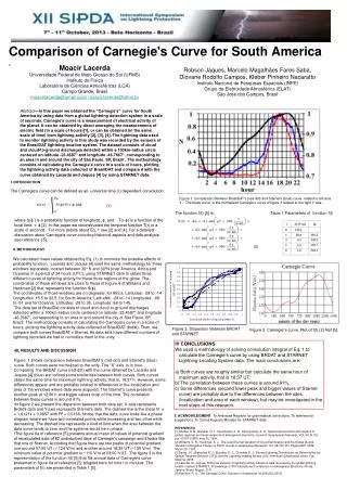
Comparison of Carnegie's Curve for South America. Moacir Lacerda Universidade Federal de Mato Grosso do Sul (UFMS) Instituto de Física Laboratório de Ciências Atmosféricas (LCA) Campo Grande, Brasil moacirlacerda@gmail.com; moacir.lacerda@ufms.br Robson Jaques, Marcelo Magalhães Fares Saba, Diovane Rodolfo Campos, Kleber Pinheiro Nacaratto Instituto Nacional de Pesquisas Espaciais (INPE) Grupo de Eletricidade Atmosférica (ELAT) São José dos Campos, Brasil Abstract—In this paper we obtained the “Carnegie's” curve for South America by using data from a global lightning detection system in a scale of seconds. Carnegie's curve is a measurement of electrical activity of the planet. It can be obtained by direct averaging the measurements of electric field (in a scale of hours)[1], or can be obtained (in the same scale of time) from lightning activity [2], [3], [4]. The lightning data used to monitor lightning activity in this study was recorded by the sensors of the BrasilDAT lightning location system. The dataset consists of cloud and cloud-to-ground discharges detected within a 100km-radius circle centered on latitude -23.4587° and longitude -46.7667°, corresponding to an area in and around the city of São Paulo, SP, Brazil . The methodology consists of calculating the Carnegie's curve in a scale of hours, plotting the lightning activity data collected of BrasilDAT and compare it with the curve obtained by Lacerda and Jaques [4] by using STARNET data. I. INTRODUCTION The Carnegie's curve can be defined as an universal time (τ) dependent convolution: (1) where S(ϕ ) is a probability function of longitude, ϕ, and T(τ-ϕ) is a function of the local time, τ- ϕ [2]. In this paper we reconstructed the temporal function T(τ) in a scale of seconds. For more details about Eq. 1 see [2] and [4]. For a detailed discussion about Carnegie's curve including historical aspects and data analysis, see reference [5]. Figure 1. Comparison Between BrasilDAT's (red-dot) and Starnet's (blue) curve related to left axis Y . The black curve is the normalized Carnegie’s curve of figure 3 related to the right Y axis. The function f(t) [5] is: Table 1 Parameters of function f(t) (2) II. METHODOLOGY We calculated mean values obtained by Eq. (1) to minimize the possible effects of probability function. Lacerda and Jaques [4] used the same methodology for three windows separately, located between 30o S and 30oN (over America, Africa and Oceania) in a period of 24 hours (UTC), using STARNET data to obtain three different curves of lightning activity for these three regions of the globe. The coordinates of these windows are close to those of Figure 4 of Williams and Heckman [2] that represents the function S(ϕ). The coordinates of those windows are (in degrees): for Africa, Latitudes: -28 to -14 Longitudes: 15.5 to 32.5; for South America: Latitudes: -28 to -14 Longitudes: -68 to -51 and for Oceania: Latitudes: -28 to 26, Longitude: 88 to 145. The data set of BrasilDat consists of cloud and cloud-to-ground discharges detected within a 100km-radius circle centered on latitude -23.4587° and longitude -46.7667°, corresponding to an area in and around the city of São Paulo, SP, Brazil. The methodology consists of calculating the Carnegie's curve in a scale of hours, plotting the lightning activity data collected of BrasilDAT (brdat). Then, we compare both curves BrasilDAT x Starnet. As data sets have different numbers of lightning recorded we had to normalize them to the unity. Figure 2. Dispersion Between BRDAT and STARNET Figure 3. Carnegie”s curve. Plot of f(t) (2) Ref [5]. eq (2) IV CONCLUSIONS We used a methodology of solving convolution integral of Eq. 1 to calculate the Carnegie’s curve by using BRDAT and STARNET Lightning Locating System data. The main conclusions are: a) Both curves are roughly similar but calculate the same hour of maximum activity, that is 18:37 UT. b) The correlation between these curves is around 91%. c) Some differences (second lower peak and bigger values of Starnet curve) are probably due to the differences between the sites (localization and area of each window), but may be investigated in the next steps of this research. • III. RESULTS AND DISCUSSION • Figure. 1 shows comparison between BrasilDAT's (red-dot) and Starnet's (blue) curve. Both curves were normalized to the unity. The "X" axis is in hour. • Comparing the BRDAT curve (red-dot) with the curve obtained by Lacerda and Jaques [4] (blue) we noticed some similarities between both curves. Both curves obtain the same time for maximum lightning activity, that is, 18:37 h. However, some differences appear and are probably related to differences in the localization and area of the windows where data were acquired. The Starnet's curve presents another peak at 12:06 h and bigger values most of the time. The correlation between these curves is around 91%. • In figure 2 we present the dispersion between both data set. X-axis represents Brdat's data and Y-axis represents Starnet's data. The dashed line is the linear fit y = 1.0121x + 0.0857 with R2 = 0.9166. Notice that the data curve looks like a phase diagram where we have two correlated points while increasing and two other while decreasing. The dashed line represents a kind of limit when the area between the data curve tends to zero and the systems would be in phase. • The figure 6a of reference [5] presents annual mean of values of potential gradient of recalculated data of 82 undisturbed days of Carnegie’s campaign and it looks like that one of Starnet. According that figure there are two peaks of potential gradient, one around 07:00 UT (~ 124 V/m) and another around 18:30 UT (~155 V/m). The minimum value of potential gradient is ~110 V/m at 03:00 h UT. The figure 3 is the representation of the function f(t) [5] that fits annual data of Carnegie's curve presented in figure 6a of reference [5] adapted here for time t in minutes. The parameters of f(t) are presented in Table 1 [5]. 5. ACKNOWLEGMENT. To Andressa Regnold for grammatical corrections. To referees for suggestions. To Carlos Augusto Morales for STARNET data. REFERENCES [1] Sheftel, V. M., Bandilet, O. I., Yaroshenko, A. N., Chernysshev, A. K., Space-time structure and reasons of global, regional, and local variations of atmospheric electricity, Jounal of Geophysical Research, VOL 99, N. D5, p.p. 10797-10806, may 20, 1994. [2] Williams, E. R., Heckman, S. J., The Local Diurnal Variation of Cloud Eletrification and the Global Diurnal Variation of Negative Charge on Earth, Jounal of Geophysical Research, Vol. 98, NO. D3, Pages 5221-5234, March 20, 1993 [3] Bailey J.C.; Blakeslee R. J.; Buechler D. E.; Christian H. J.; Diurnal Lightning Distributions as Observed by the Optical Transient Detector (OTD) and the Lightning Imaging Sensor (LIS); American Geophysical Union, Fall Meeting, 2006. [4] Lacerda, M., Jaques, R Diurnal variation of lightning activity based on data recorded by the global lightning location system STARNET., Proceedings of XIV International Conference on Atmospheric Electricity, Rio de Janeiro, Brazil, August, 2011. [5] Harrison, R. G., The Carnegie Curve, Surveys in Geophysics 34:209-232 (2013).